# 安装包
if (!requireNamespace("ggplot2", quietly = TRUE)) {
  install.packages("ggplot2")
}
if (!requireNamespace("ggisoband", quietly = TRUE)) {
  install.packages("ggisoband")
}

# 加载包
library(ggplot2)
library(ggisoband)等高线图 (XY)
注记
Hiplot 网站
本页面为 Hiplot Contour (XY) 插件的源码版本教程,您也可以使用 Hiplot 网站实现无代码绘图,更多信息请查看以下链接:
等高线图 (XY) 是一种通过等高线反映数据密集程度的数据处理方式。
环境配置
系统: Cross-platform (Linux/MacOS/Windows)
编程语言: R
依赖包:
ggplot2;ggisoband
数据准备
载入数据为两个变量。
# 加载数据
data <- read.delim("files/Hiplot/028-contour-xy-data.txt", header = T)

# 整理数据格式
colnames(data) <- c("xvalue", "yvalue")

# 查看数据
head(data)
xvalue yvalue
1 2.620 110
2 2.875 110
3 2.320 93
4 3.215 110
5 3.440 175
6 3.460 105可视化
# 等高线图 (XY)
p <- ggplot(data, aes(xvalue, yvalue)) +
  geom_density_bands(
    alpha = 1,
    aes(fill = stat(density)), color = "gray40", size = 0.2
    ) +
  geom_point(alpha = 1, shape = 21, fill = "white") +
  scale_fill_viridis_c(guide = "legend") +
  ylab("value2") +
  xlab("value1") +
  ggtitle("Contour-XY Plot") +
  theme_bw() +
  theme(text = element_text(family = "Arial"),
        plot.title = element_text(size = 12,hjust = 0.5),
        axis.title = element_text(size = 12),
        axis.text = element_text(size = 10),
        axis.text.x = element_text(angle = 0, hjust = 0.5,vjust = 1),
        legend.position = "right",
        legend.direction = "vertical",
        legend.title = element_text(size = 10),
        legend.text = element_text(size = 10))

p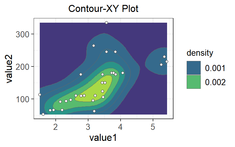
正如地理上的等高线代表不同高度一样,等高线图上的不同等高线代表不同密度,越靠中心,等高线圈越小,代表其区域数据密度程度越高。如:黄色区域数据密集程度最高,而蓝色区域数据密集程度最低。