Chi-square-fisher Test

Authors

[Editor] Hu Zheng;

[Contributors]

Chi-square and Fisher test can be used to test the frequency difference of categorical variables. The tool will automatically select the statistical method of Chi-square and Fisher exact test.

Setup

System Requirements: Cross-platform (Linux/MacOS/Windows)
Programming language: R
Dependent packages: ggplot2; visdat; aplot

# Install packages
if (!requireNamespace("ggplot2", quietly = TRUE)) {
  install.packages("ggplot2")
}
if (!requireNamespace("visdat", quietly = TRUE)) {
  install.packages("visdat")
}
if (!requireNamespace("aplot", quietly = TRUE)) {
  install.packages("aplot")
}

# Load packages
library(ggplot2)
library(visdat)
library(aplot)

Data Preparation

The data table supports two formats: contingency table (example 1) and single-row record table (example 2)

# Load data
data <- read.table("files/Hiplot/019-chi-square-fisher-data.txt", header = T)

# convert data structure
rownames(data) <- data[,1]
data <- data[,-1]
cb <- combn(nrow(data), 2)
final <- data.frame()
for (i in 1:ncol(cb)) {
  tmp <- data[cb[,i],]
  groups <- paste0(rownames(data)[cb[,i]], collapse = " | ")
  
  res <- tryCatch({
    chisq.test(tmp)
    }, warning = function(w) {
      tryCatch({fisher.test(tmp)}, error = function(e) {
        return(fisher.test(tmp, simulate.p.value = TRUE))
        })
  })
  val_percent <- apply(tmp, 1, function(x) {
    sprintf("%s (%s%%)", x, round(x / sum(x), 2) * 100)
  })
  val_percent1 <- paste0(colnames(tmp), ":", val_percent[,1])
  val_percent1 <- paste0(val_percent1, collapse = " | ")
  val_percent2 <- paste0(colnames(tmp), ":", val_percent[,2])
  val_percent2 <- paste0(val_percent2, collapse = " | ")
  tmp <- data.frame(
    groups = groups,
    val_percent_left = val_percent1,
    val_percent_right = val_percent2,
    statistic = ifelse(is.null(res$statistic), NA,
      as.numeric(res$statistic)),
    pvalue = as.numeric(res$p.value),
    method = res$method
  )
  final <- rbind(final, tmp)
}
final <- as.data.frame(final)
final$pvalue < as.numeric(final$pvalue)

 [1] FALSE FALSE FALSE FALSE FALSE FALSE FALSE FALSE FALSE FALSE

final$statistic < as.numeric(final$statistic)

 [1] FALSE FALSE FALSE    NA FALSE FALSE    NA FALSE    NA    NA

# View data
head(final)

  groups                        val_percent_left
1  A | B L:401 (48%) | M:216 (26%) | H:221 (26%)
2  A | C L:401 (48%) | M:216 (26%) | H:221 (26%)
3  A | D L:401 (48%) | M:216 (26%) | H:221 (26%)
4  A | E L:401 (48%) | M:216 (26%) | H:221 (26%)
5  B | C L:254 (37%) | M:259 (38%) | H:169 (25%)
6  B | D L:254 (37%) | M:259 (38%) | H:169 (25%)
                        val_percent_right    statistic       pvalue
1 L:254 (37%) | M:259 (38%) | H:169 (25%) 2.810229e+01 7.900708e-07
2 L:400 (48%) | M:215 (26%) | H:220 (26%) 4.566425e-04 9.997717e-01
3 L:252 (38%) | M:251 (38%) | H:162 (24%) 2.614390e+01 2.103411e-06
4       L:3 (23%) | M:5 (38%) | H:5 (38%)           NA 1.633146e-01
5 L:400 (48%) | M:215 (26%) | H:220 (26%) 2.821998e+01 7.449197e-07
6 L:252 (38%) | M:251 (38%) | H:162 (24%) 6.689139e-02 9.671074e-01
                              method
1         Pearson's Chi-squared test
2         Pearson's Chi-squared test
3         Pearson's Chi-squared test
4 Fisher's Exact Test for Count Data
5         Pearson's Chi-squared test
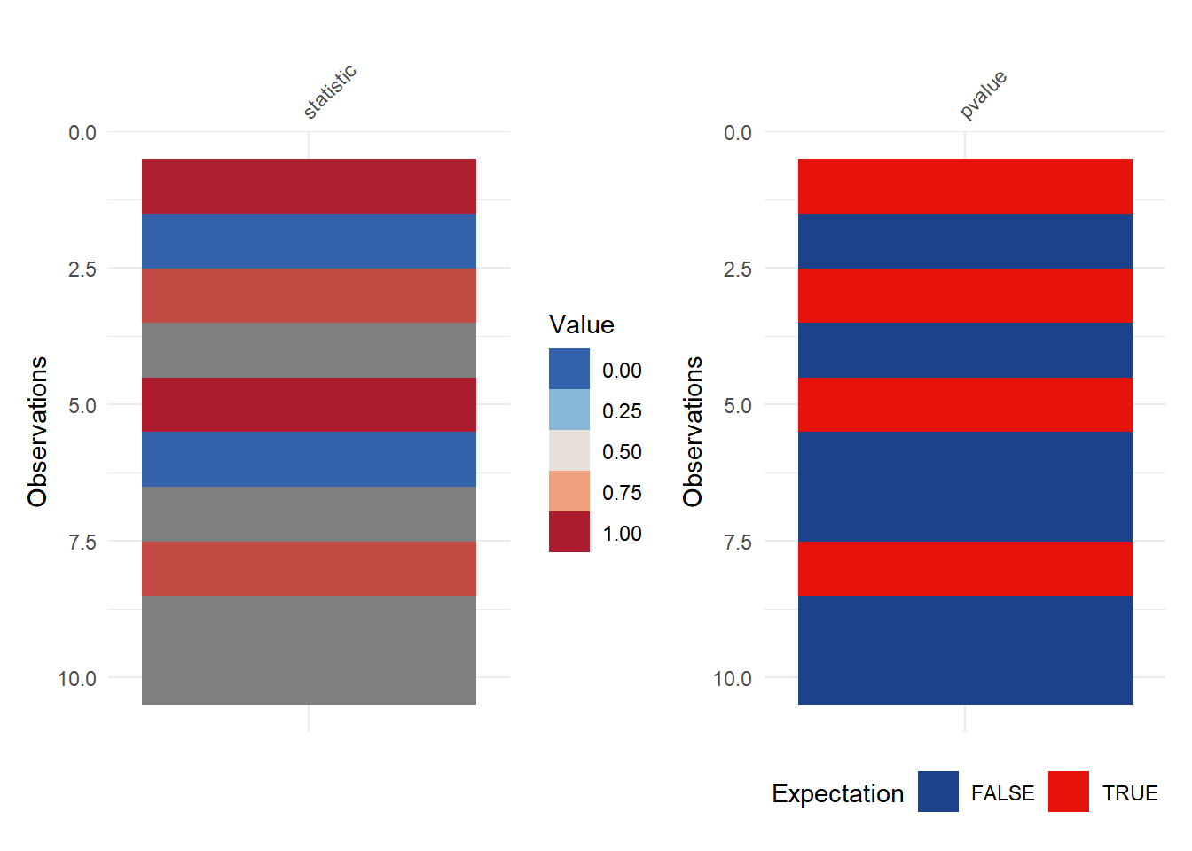
6         Pearson's Chi-squared test

Visualization

# Chi-square-fisher Test
p1 <- vis_value(final["statistic"]) + 
  scale_fill_gradientn(colours = c("#3362ab","#87b7d7","#e8e0db","#eea07d","#ad1c2e"))

p2 <- vis_expect(final["pvalue"], ~.x < 0.05) +
  scale_fill_manual(values = c("#1c438a","#e7120c"))

p <- p1+p2
p