Extended Scatter

Authors

[Editor] Hu Zheng;

[Contributors]

Note

Hiplot website

This page is the tutorial for source code version of the Hiplot Extended Scatter plugin. You can also use the Hiplot website to achieve no code ploting. For more information please see the following link:

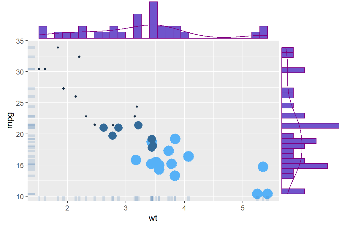
https://hiplot.cn/basic/extended-scatter?lang=en

An extended scatter plot adds marginal plots to the basic scatter plot to provide a more comprehensive view of the data distribution.

Setup

System Requirements: Cross-platform (Linux/MacOS/Windows)
Programming language: R
Dependent packages: ggplot2; ggExtra

# Install packages
if (!requireNamespace("ggplot2", quietly = TRUE)) {
  install.packages("ggplot2")
}
if (!requireNamespace("ggExtra", quietly = TRUE)) {
  install.packages("ggExtra")
}

# Load packages
library(ggplot2)
library(ggExtra)

Data Preparation

# Load data
data <- read.delim("files/Hiplot/052-extended-scatter-data.txt", header = T)

# View data
head(data)

   mpg cyl disp  hp drat    wt  qsec vs am gear carb
1 21.0   6  160 110 3.90 2.620 16.46  0  1    4    4
2 21.0   6  160 110 3.90 2.875 17.02  0  1    4    4
3 22.8   4  108  93 3.85 2.320 18.61  1  1    4    1
4 21.4   6  258 110 3.08 3.215 19.44  1  0    3    1
5 18.7   8  360 175 3.15 3.440 17.02  0  0    3    2
6 18.1   6  225 105 2.76 3.460 20.22  1  0    3    1

Visualization

# Extended Scatter
p <- ggplot(data, aes(x = wt, y = mpg, color = cyl, size = cyl)) +
  geom_point() +
  geom_rug(alpha = 0.2, size = 1.5, col = "#4f80b3") +
  theme(legend.position = "none")

p <- ggMarginal(
  p, type = "densigram", fill = "#7054cc", color = "#7f0080",
  size = 4, bins = 30)

p