# Install packages
if (!requireNamespace("kohonen", quietly = TRUE)) {
  install.packages("kohonen")
}

# Load packages
library(kohonen)Easy SOM
Note
Hiplot website
This page is the tutorial for source code version of the Hiplot Easy SOM plugin. You can also use the Hiplot website to achieve no code ploting. For more information please see the following link:
Establish the SOM model and conduct the visulization.
Setup
System Requirements: Cross-platform (Linux/MacOS/Windows)
Programming language: R
Dependent packages:
kohonen
Data Preparation
# Load data
data <- read.delim("files/Hiplot/050-easy-som-data.txt", header = T)

# convert data structure
target <- data[,1]
target <- factor(target, levels = unique(target))
data <- data[,-1]
data <- as.data.frame(data)
for (i in 1:ncol(data)) {
  data[,i] <- as.numeric(data[,i])
}
data <- as.matrix(data)
set.seed(7)
kohmap <- xyf(scale(data), target, grid = somgrid(xdim=6, ydim=4, topo="hexagonal"), rlen=100)

color_key <- c("#A50026","#D73027","#F46D43","#FDAE61","#FEE090","#FFFFBF","#E0F3F8",
               "#ABD9E9","#74ADD1","#4575B4","#313695")
colors <- function (n, alpha, rev = FALSE) {
  colorRampPalette(color_key)(n)
}

# View data
head(data)
alcohol malic.acid ash ash.alkalinity magnesium tot..phenols flavonoids
[1,] 12.86 1.35 2.32 18.0 122 1.51 1.25
[2,] 12.88 2.99 2.40 20.0 104 1.30 1.22
[3,] 12.81 2.31 2.40 24.0 98 1.15 1.09
[4,] 12.70 3.55 2.36 21.5 106 1.70 1.20
[5,] 12.51 1.24 2.25 17.5 85 2.00 0.58
[6,] 12.60 2.46 2.20 18.5 94 1.62 0.66
non.flav..phenols proanth col..int. col..hue OD.ratio proline
[1,] 0.21 0.94 4.10 0.76 1.29 630
[2,] 0.24 0.83 5.40 0.74 1.42 530
[3,] 0.27 0.83 5.70 0.66 1.36 560
[4,] 0.17 0.84 5.00 0.78 1.29 600
[5,] 0.60 1.25 5.45 0.75 1.51 650
[6,] 0.63 0.94 7.10 0.73 1.58 695Visualization
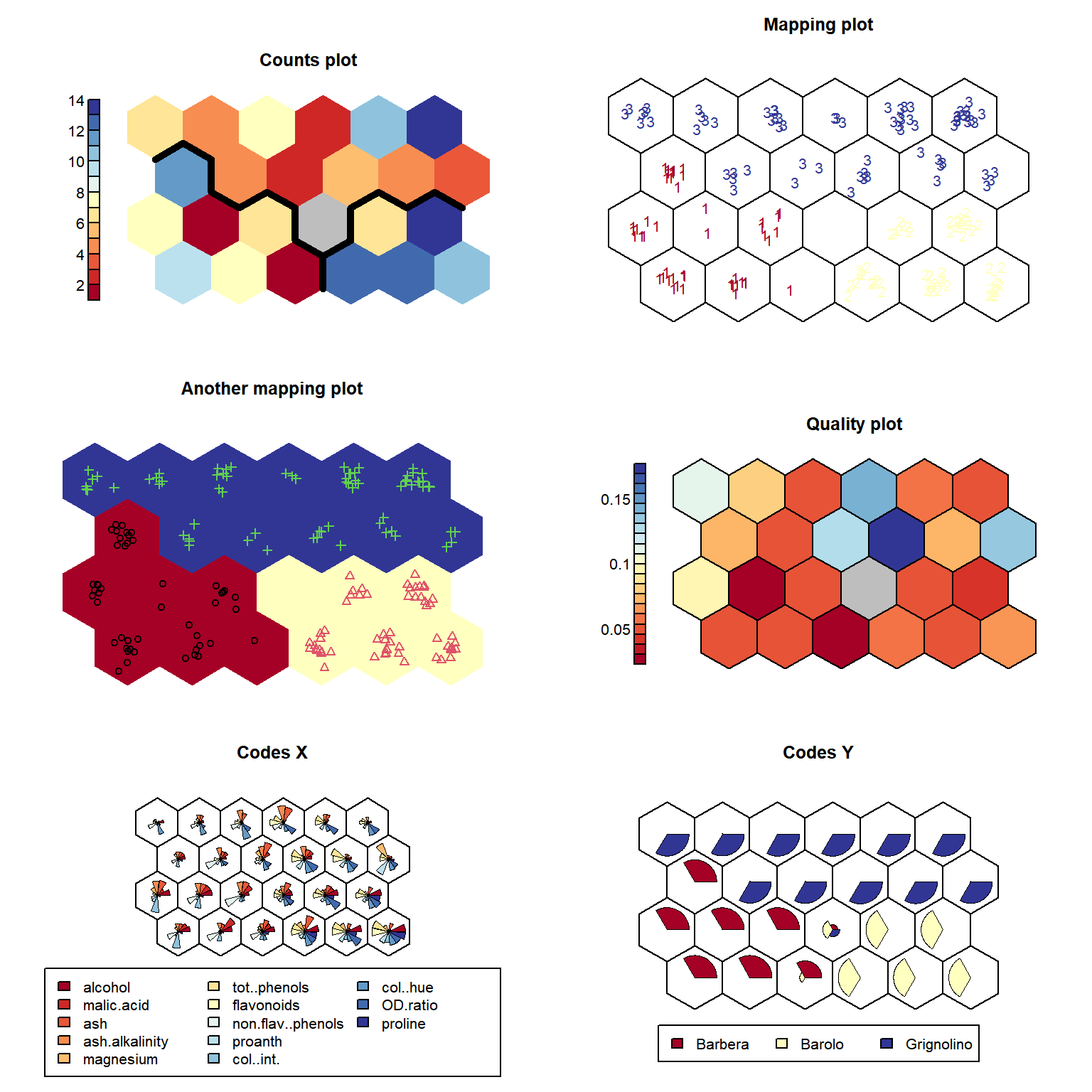
# Easy SOM
p <- function () {
  par(mfrow = c(3,2))
  xyfpredictions <- classmat2classvec(getCodes(kohmap, 2))
  plot(kohmap, type="counts", col = as.integer(target),
       palette.name = colors,
       pchs = as.integer(target),
       main = "Counts plot", shape = "straight", border = NA)

  som.hc <- cutree(hclust(object.distances(kohmap, "codes")), 3)
  add.cluster.boundaries(kohmap, som.hc)

  plot(kohmap, type="mapping",
       labels = as.integer(target), col = colors(3)[as.integer(target)],
       palette.name = colors,
       shape = "straight",
       main = "Mapping plot")

  ## add background colors to units according to their predicted class labels
  xyfpredictions <- classmat2classvec(getCodes(kohmap, 2))
  bgcols <- colors(3)
  plot(kohmap, type="mapping", col = as.integer(target),
       pchs = as.integer(target), bgcol = bgcols[as.integer(xyfpredictions)],
       main = "Another mapping plot", shape = "straight", border = NA)

  similarities <- plot(kohmap, type="quality", shape = "straight",
                       palette.name = colors)

  plot(kohmap, type="codes", shape = "straight",
       main = c("Codes X", "Codes Y"), palette.name = colors)
}

p()