Directed Acyclic Graphs

Authors

[Editor] Hu Zheng;

[Contributors]

Note

Hiplot website

This page is the tutorial for source code version of the Hiplot Directed Acyclic Graphs plugin. You can also use the Hiplot website to achieve no code ploting. For more information please see the following link:

https://hiplot.cn/basic/ggdag?lang=en

Visualizing directed acyclic graphs.

Setup

System Requirements: Cross-platform (Linux/MacOS/Windows)
Programming language: R
Dependent packages: ggdag

# Install packages
if (!requireNamespace("ggdag", quietly = TRUE)) {
  install.packages("ggdag")
}

# Load packages
library(ggdag)

Data Preparation

# Load data
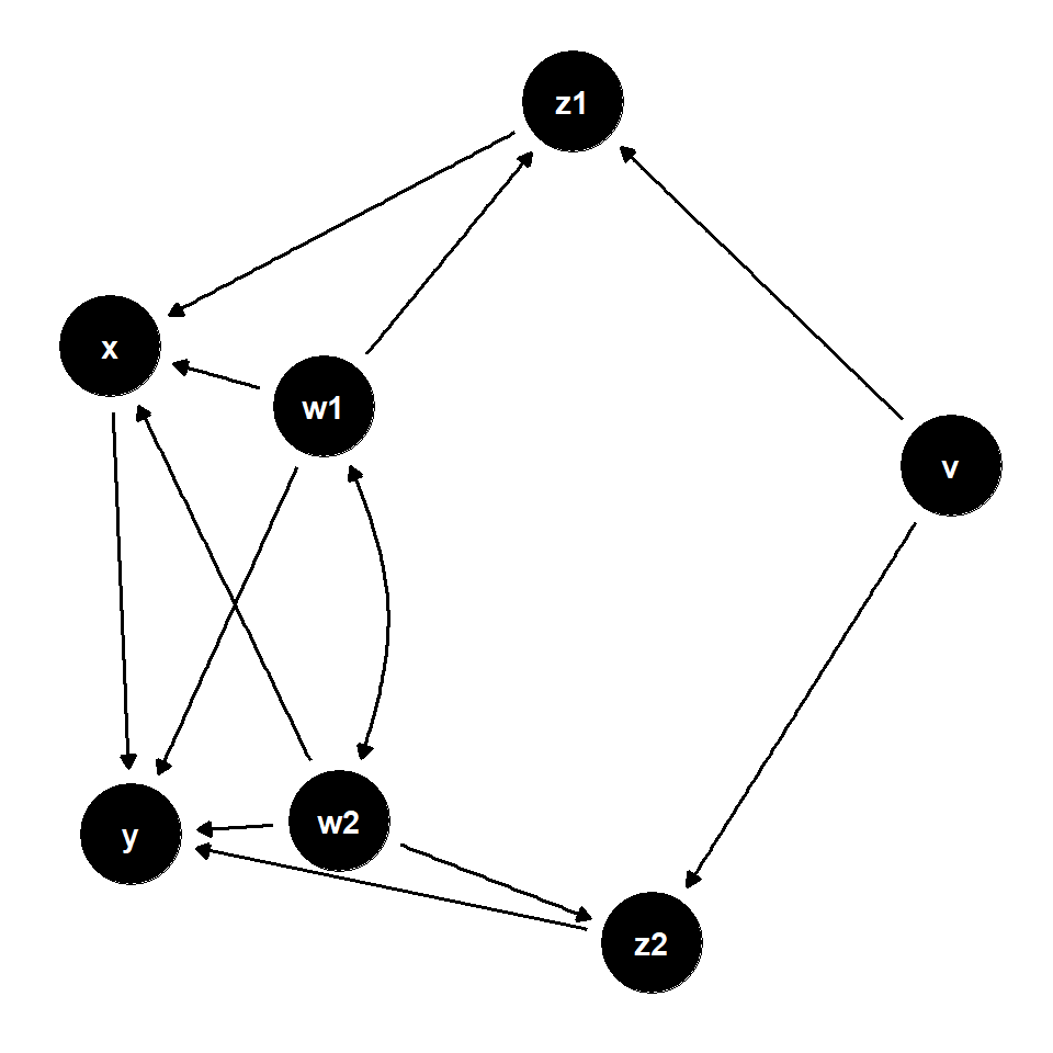
tidy_ggdag <- dagify(
  y ~ x + z2 + w2 + w1,
  x ~ z1 + w1 + w2,
  z1 ~ w1 + v,
  z2 ~ w2 + v,
  w1 ~ ~w2, # bidirected path
  exposure = "x",
  outcome = "y") %>%
  tidy_dagitty()

# View data
head(tidy_ggdag)

$data
# A tibble: 13 × 8
   name        x      y direction to       xend   yend circular
   <chr>   <dbl>  <dbl> <fct>     <chr>   <dbl>  <dbl> <lgl>   
 1 v     -1.49    0.461 ->        z1    -0.0837  0.635 FALSE   
 2 v     -1.49    0.461 ->        z2    -1.34   -0.944 FALSE   
 3 w1     0.232  -0.302 ->        x      0.791  -0.591 FALSE   
 4 w1     0.232  -0.302 ->        y      0.0525 -1.50  FALSE   
 5 w1     0.232  -0.302 ->        z1    -0.0837  0.635 FALSE   
 6 w1     0.232  -0.302 <->       w2    -0.364  -1.03  FALSE   
 7 w2    -0.364  -1.03  ->        x      0.791  -0.591 FALSE   
 8 w2    -0.364  -1.03  ->        y      0.0525 -1.50  FALSE   
 9 w2    -0.364  -1.03  ->        z2    -1.34   -0.944 FALSE   
10 x      0.791  -0.591 ->        y      0.0525 -1.50  FALSE   
11 y      0.0525 -1.50  <NA>      <NA>  NA      NA     FALSE   
12 z1    -0.0837  0.635 ->        x      0.791  -0.591 FALSE   
13 z2    -1.34   -0.944 ->        y      0.0525 -1.50  FALSE   

$dag
dag {
v
w1
w2
x [exposure]
y [outcome]
z1
z2
v -> z1
v -> z2
w1 -> x
w1 -> y
w1 -> z1
w1 <-> w2
w2 -> x
w2 -> y
w2 -> z2
x -> y
z1 -> x
z2 -> y
}

Visualization

# Directed Acyclic Graphs
p <- ggdag(tidy_ggdag) +
  theme_dag() 

p