# Install packages
if (!requireNamespace("ape", quietly = TRUE)) {
  install.packages("ape")
}
if (!requireNamespace("ggplotify", quietly = TRUE)) {
  install.packages("ggplotify")
}

# Load packages
library(ape)
library(ggplotify)Dendrogram
Note
Hiplot website
This page is the tutorial for source code version of the Hiplot Dendrogram plugin. You can also use the Hiplot website to achieve no code ploting. For more information please see the following link:
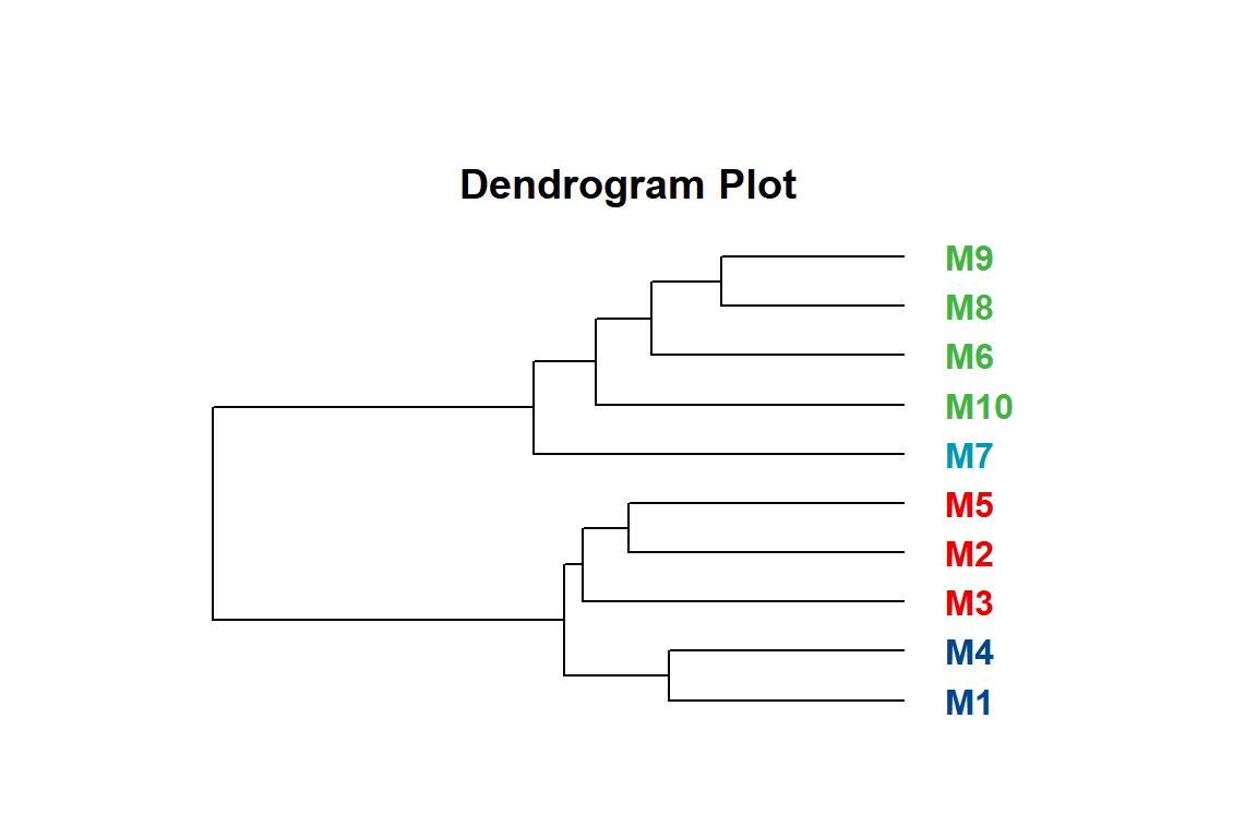
The dendrogram is a diagram representing a tree. This diagrammatic representation is frequently used in different contexts:In hierarchical clustering, it illustrates the arrangement of the clusters produced by the corresponding analyses.
Setup
System Requirements: Cross-platform (Linux/MacOS/Windows)
Programming language: R
Dependent packages:
ape;ggplotify
Data Preparation
# Load data
data <- read.delim("files/Hiplot/037-dendrogram-data.txt", header = T)

# convert data structure
data <- data[, -1]

# View data
head(data)
M1 M2 M3 M4 M5 M6 M7 M8
1 6.599344 5.226266 3.693288 3.938501 4.527193 9.308119 8.987865 7.658312
2 5.760380 4.892783 5.448924 3.485413 3.855669 8.662081 8.793320 8.765915
3 9.561905 4.549168 3.998655 5.614384 3.904793 9.790770 7.133188 7.379591
4 8.396409 8.717055 8.039064 7.643060 9.274649 4.417013 4.725270 3.542217
5 8.419766 8.268430 8.451181 9.200732 8.598207 4.590033 5.368268 4.136667
6 7.653074 5.780393 10.633550 5.913684 8.805605 5.890120 5.527945 3.822596
M9 M10
1 8.666038 7.419708
2 8.097206 8.262942
3 7.938063 6.154118
4 4.305187 6.964710
5 4.910986 4.080363
6 4.041078 7.956589Visualization
# Dendrogram
d <- dist(t(data), method = "euclidean")
hc <- hclust(d, method = "complete")
clus <- cutree(hc, 4)

p <- as.ggplot(function() {
  par(mar = c(5, 5, 10, 5), mgp = c(2.5, 1, 0))
  plot(as.phylo(hc),
       type = "phylogram",
       tip.color = c("#00468bff","#ed0000ff","#42b540ff","#0099b4ff")[clus],
       label.offset = 1,
       cex = 1, font = 2, use.edge.length = T
       )
  title("Dendrogram Plot", line = 1)
  })

p