# Install packages
if (!requireNamespace("ggdist", quietly = TRUE)) {
  install.packages("ggdist")
}
if (!requireNamespace("tidyr", quietly = TRUE)) {
  install.packages("tidyr")
}
if (!requireNamespace("broom", quietly = TRUE)) {
  install.packages("broom")
}
if (!requireNamespace("modelr", quietly = TRUE)) {
  install.packages("modelr")
}
if (!requireNamespace("ggplot2", quietly = TRUE)) {
  install.packages("ggplot2")
}

# Load packages
library(ggdist)
library(tidyr)
library(broom)
library(modelr)
library(ggplot2)Dist Plot
Note
Hiplot website
This page is the tutorial for source code version of the Hiplot Dist Plot plugin. You can also use the Hiplot website to achieve no code ploting. For more information please see the following link:
The dist plot is a visual diagram using a confidence distribution.
Setup
System Requirements: Cross-platform (Linux/MacOS/Windows)
Programming language: R
Dependent packages:
ggdist;tidyr;broom;modelr;ggplot2
Data Preparation
The loaded data are five conditions and their corresponding values.
# Load data
data <- read.delim("files/Hiplot/066-ggdist-data.txt", header = T)

# Convert data structure
data[, 1] <- factor(data[, 1], levels = rev(unique(data[, 1])))
data <- tibble(data)
data2 = lm(response ~ condition, data = data)
data3 <- data_grid(data, condition) %>%
  augment(data2, newdata = ., se_fit = TRUE)

# View data
head(data)
# A tibble: 6 × 2
condition response
<fct> <dbl>
1 A -0.420
2 B 1.69
3 C 1.37
4 D 1.04
5 E -0.144
6 A -0.301Visualization
# Dist Plot
p <- ggplot(data3, aes_(y = as.name(colnames(data[1])))) +
  stat_dist_halfeye(aes(dist = "student_t", arg1 = df.residual(data2),
                        arg2 = .fitted, arg3 = .se.fit),
                    scale = .5) +
  geom_point(aes_(x = as.name(colnames(data[2]))),
             data = data, pch = "|", size = 2,
             position = position_nudge(y = -.15)) +
  ggtitle("ggdist Plot") +
  xlab("response") + ylab("condition") +
  theme_ggdist() +
  theme(text = element_text(family = "Arial"),
        plot.title = element_text(size = 12,hjust = 0.5),
        axis.title = element_text(size = 12),
        axis.text = element_text(size = 10),
        axis.text.x = element_text(angle = 0, hjust = 0.5,vjust = 1),
        legend.position = "right",
        legend.direction = "vertical",
        legend.title = element_text(size = 10),
        legend.text = element_text(size = 10))

p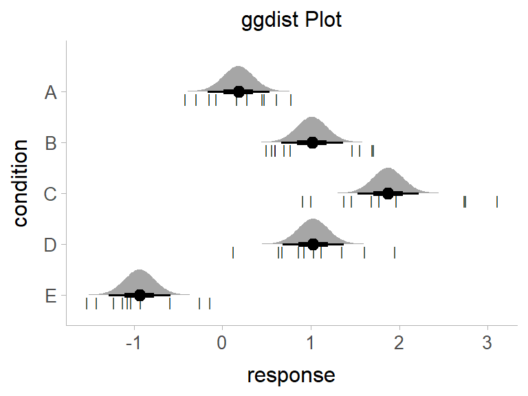
The diagram shows the confidence distribution of the mean under the conditions, and the approximate distribution of the corresponding values under the five conditions can be seen.