# Installing necessary packages
if (!requireNamespace("MetaNet", quietly = TRUE)) {
  install.packages("MetaNet")
}
if (!requireNamespace("pcutils", quietly = TRUE)) {
  install.packages("pcutils")
}
if (!requireNamespace("igraph", quietly = TRUE)) {
  install.packages("igraph")
}
if (!requireNamespace("dplyr", quietly = TRUE)) {
  install.packages("dplyr")
}

# Load packages
library(MetaNet)
library(pcutils)
library(igraph)
library(dplyr)Network Plot
In microbiome research, it is crucial to understand the interactions between microorganisms. Network analysis is a powerful method that can help us visualize and quantify these complex relationships. Next, we will introduce the network operation and annotation functions of the MetaNet package, which can make our network analysis more in-depth and intuitive.
Example
Setup
System Requirements: Cross-platform (Linux/MacOS/Windows)
Programming language: R
Dependent packages:
MetaNet;pcutils;igraph;dplyr
Data Preparation
1. Load data
- The data uses the
otutabdataset in pcutils - MetaNet is an R package for comprehensive network analysis of omics data
- The
c_net_calculate()function is used to quickly calculate the correlation between variables - The
c_net_build()function is used to build the network
data(otutab, package = "pcutils")
t(otutab) -> totu
c_net_calculate(totu, method = "spearman") -> corr
c_net_build(corr, r_threshold = 0.6, p_threshold = 0.05, delete_single = T) -> co_net
class(co_net)
[1] "metanet" "igraph" 2. Get network properties
After building a network with MetaNet, you get a classification object, which comes from igraph. This means that you can use MetaNet’s proprietary functions and igraph’s general functions at the same time. Next, learn how to get basic information about the network:
# Get overall network properties
get_n(co_net)
n_type
1 single# View node properties
get_v(co_net) %>% head(5) name v_group v_class size
1 s__un_f__Thermomonosporaceae v_group1 v_class1 4
2 s__Pelomonas_puraquae v_group1 v_class1 4
3 s__Rhizobacter_bergeniae v_group1 v_class1 4
4 s__Flavobacterium_terrae v_group1 v_class1 4
5 s__un_g__Rhizobacter v_group1 v_class1 4
label shape color
1 s__un_f__Thermomonosporaceae circle #a6bce3
2 s__Pelomonas_puraquae circle #a6bce3
3 s__Rhizobacter_bergeniae circle #a6bce3
4 s__Flavobacterium_terrae circle #a6bce3
5 s__un_g__Rhizobacter circle #a6bce3# View edge properties
get_e(co_net) %>% head(5) id from to weight
1 1 s__un_f__Thermomonosporaceae s__Actinocorallia_herbida 0.6759546
2 2 s__un_f__Thermomonosporaceae s__Kribbella_catacumbae 0.6742386
3 3 s__un_f__Thermomonosporaceae s__Kineosporia_rhamnosa 0.7378741
4 4 s__un_f__Thermomonosporaceae s__un_f__Micromonosporaceae 0.6236449
5 5 s__un_f__Thermomonosporaceae s__Flavobacterium_saliperosum 0.6045747
cor p.value e_type width color e_class lty
1 0.6759546 0.0020739524 positive 0.6759546 #48A4F0 e_class1 1
2 0.6742386 0.0021502138 positive 0.6742386 #48A4F0 e_class1 1
3 0.7378741 0.0004730567 positive 0.7378741 #48A4F0 e_class1 1
4 0.6236449 0.0056818984 positive 0.6236449 #48A4F0 e_class1 1
5 0.6045747 0.0078660171 positive 0.6045747 #48A4F0 e_class1 1The data frames returned by these functions contain the most basic key information of multi-omics biological networks, such as node name, grouping, size, edge weight, etc. MetaNet has set some internal attributes (such as v_group, v_class, e_type, etc.) when building the network, which will affect subsequent analysis and visualization.
3. Adding biological meaning to networks
In microbiome research, network structure alone is not enough, we need to integrate biological information such as taxonomy and abundance. MetaNet provides flexible annotation functions:
# Adding classification information to a node
c_net_annotate(co_net, taxonomy["Phylum"], mode = "v") -> co_net1
anno <- data.frame("from" = "s__un_f__Thermomonosporaceae",
                   "to" = "s__Actinocorallia_herbida", new_atr = "new")
c_net_annotate(co_net, anno, mode = "e") -> co_net1
In MetaNet, a c_net_set() function is provided, which can add multiple annotation tables at the same time and specify which columns are used to set node size, color and other attributes:
Abundance_df <- data.frame("Abundance" = colSums(totu))
co_net1 <- c_net_set(co_net, taxonomy["Phylum"], Abundance_df)
co_net1 <- co_net
V(co_net1)$new_attri <- seq_len(length(co_net1))
E(co_net1)$new_attri <- "new attribute"
get_e(co_net1) %>% head(5)
id from to weight
1 1 s__un_f__Thermomonosporaceae s__Actinocorallia_herbida 0.6759546
2 2 s__un_f__Thermomonosporaceae s__Kribbella_catacumbae 0.6742386
3 3 s__un_f__Thermomonosporaceae s__Kineosporia_rhamnosa 0.7378741
4 4 s__un_f__Thermomonosporaceae s__un_f__Micromonosporaceae 0.6236449
5 5 s__un_f__Thermomonosporaceae s__Flavobacterium_saliperosum 0.6045747
cor p.value e_type width color e_class lty new_attri
1 0.6759546 0.0020739524 positive 0.6759546 #48A4F0 e_class1 1 new attribute
2 0.6742386 0.0021502138 positive 0.6742386 #48A4F0 e_class1 1 new attribute
3 0.7378741 0.0004730567 positive 0.7378741 #48A4F0 e_class1 1 new attribute
4 0.6236449 0.0056818984 positive 0.6236449 #48A4F0 e_class1 1 new attribute
5 0.6045747 0.0078660171 positive 0.6045747 #48A4F0 e_class1 1 new attributeIn this way, a network information with both statistical significance and biological background can be obtained.
Visualization
1. Build network
Simple multi-omics network: contains information of microbiome, metabolome, transcriptome, etc.
# Basic Network
data("multi_test", package = "MetaNet")
data("c_net", package = "MetaNet")
multi1 <- multi_net_build(list(Microbiome = micro, Metabolome = metab, Transcriptome = transc))
plot(multi1)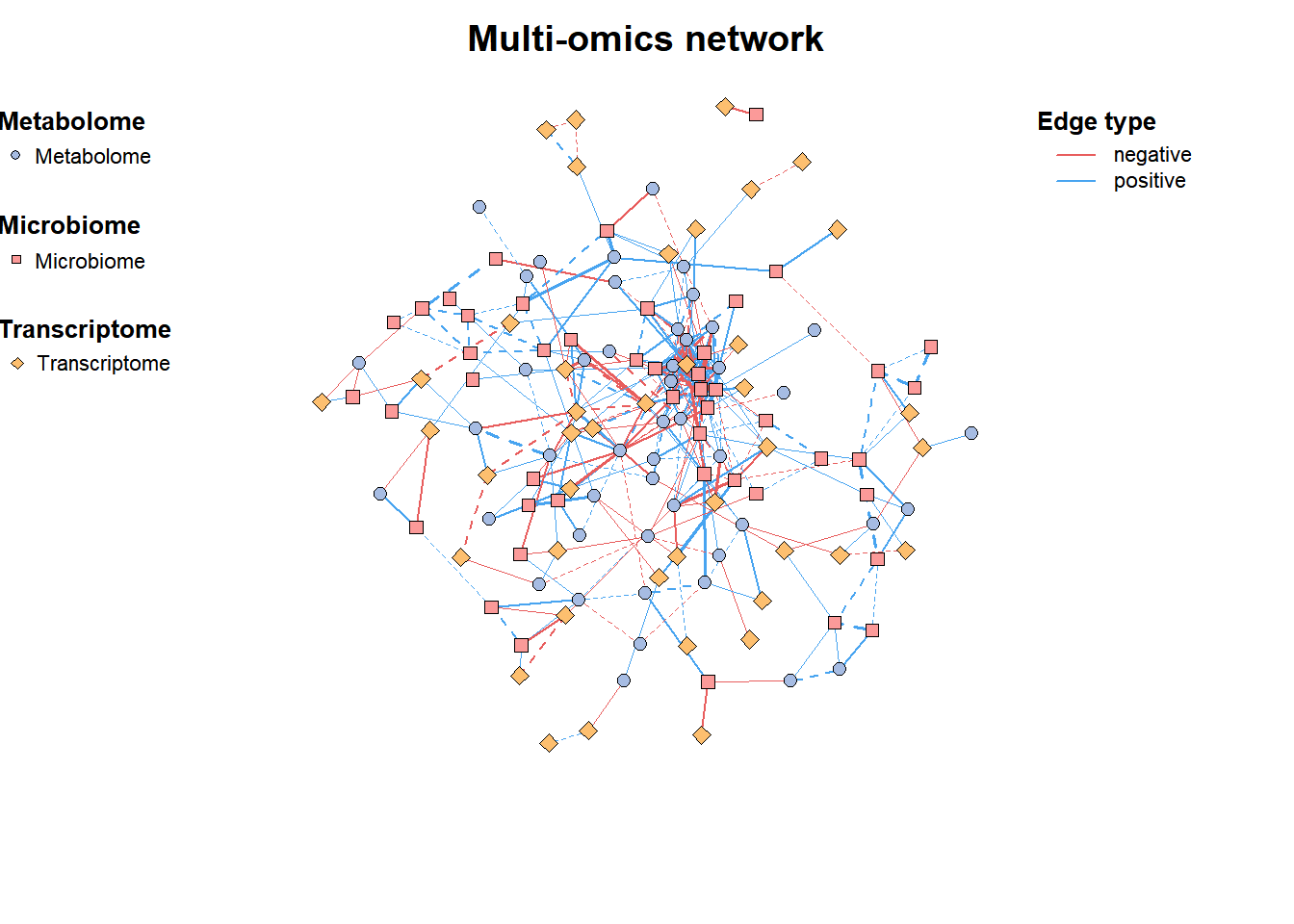
2. Add annotation
# Set the node class
multi1_with_anno <- c_net_set(multi1,
                              micro_g, metab_g,
                              transc_g,
                              vertex_class = c("Phylum", "kingdom", "type"))

# Set the node size
multi1_with_anno <- c_net_set(multi1_with_anno,
                              data.frame("Abundance1" = colSums(micro)),
                              data.frame("Abundance2" = colSums(metab)),
                              data.frame("Abundance3" = colSums(transc)),
                              vertex_size = paste0("Abundance", 1:3))

plot(multi1_with_anno)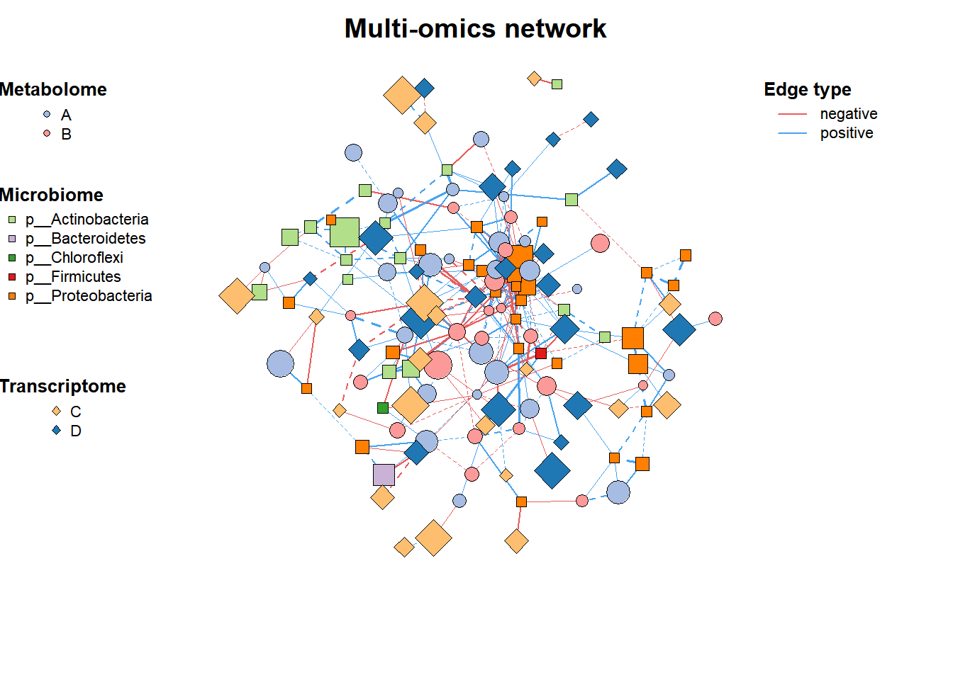
3. Filter subnetwork
# Filter subnetwork
data("multi_net", package = "MetaNet")
multi2 <- c_net_filter(multi1_with_anno, v_group %in%
                         c("Microbiome", "Metabolome")) %>%
  c_net_filter(., e_class == "intra", mode = "e")

plot(multi2, lty_legend = T, main = "Sub-network") 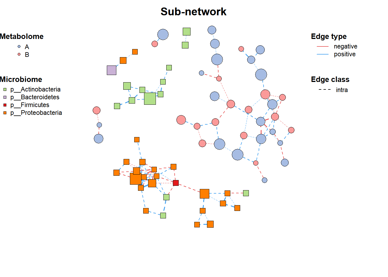
4. Merge Network
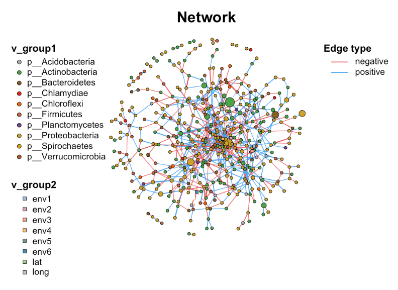
# Network1
data("c_net")
plot(co_net)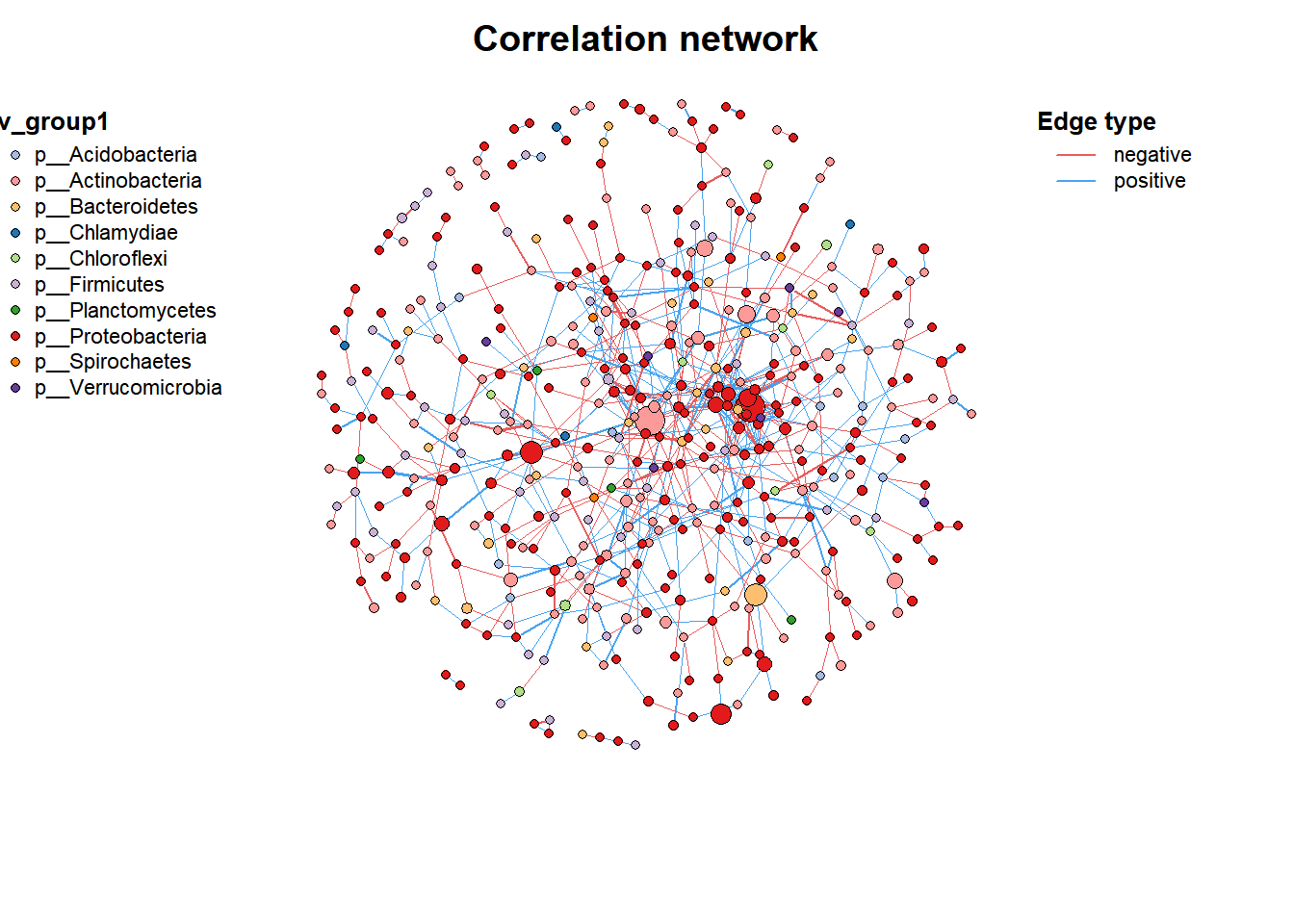
# Network2
data("c_net")
plot(co_net2)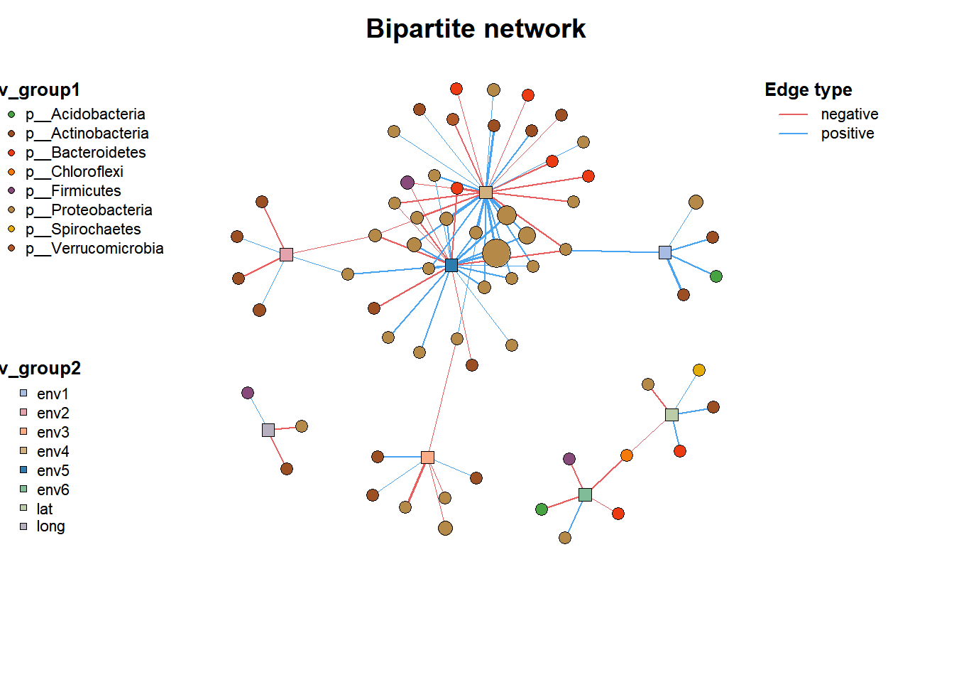
# Merge Network
co_net_union <- c_net_union(co_net, co_net2)
plot(co_net_union)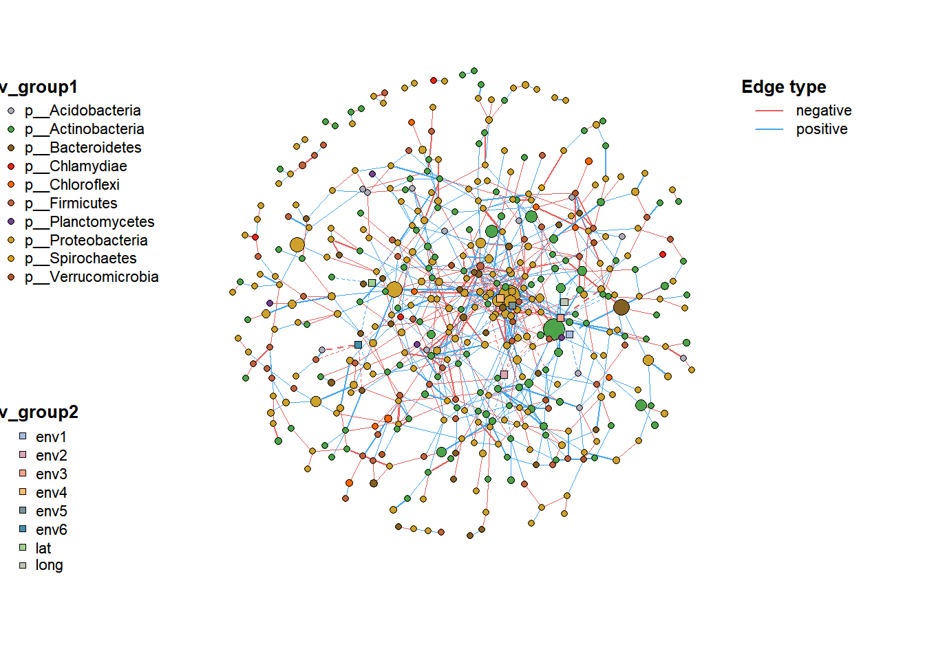
The MetaNet package provides a comprehensive set of tools for microbial network analysis, from basic network construction to advanced annotation and visualization. By flexibly using these functions, we can extract meaningful biological patterns from complex microbiome data and provide new perspectives for understanding the structure and function of microbial communities.
Reference
[1] K. Contrepois, S. Wu, K. J. Moneghetti, D. Hornburg, et al., [Molecular Choreography of Acute Exercise (https://doi.org/10.1016/j.cell.2020.04.043). Cell. 181, 1112–1130.e16 (2020).
[2] Y. Deng, Y. Jiang, Y. Yang, Z. He, et al., Molecular ecological network analyses. BMC bioinformatics (2012), doi:10.1186/1471-2105-13-113.
[3] K. Faust, J. Raes, Microbial interactions: From networks to models. Nature Reviews Microbiology (2012), doi:10.1038/nrmicro2832.
[4] Chen Peng (2025). MetaNet: Network Analysis for Omics Data. R package