Gene Density

Note

Hiplot website

This page is the tutorial for source code version of the Hiplot Gene Density plugin. You can also use the Hiplot website to achieve no code ploting. For more information please see the following link:

https://hiplot.cn/basic/gene-density?lang=en

Chrosome data visualization.

Setup

• System Requirements: Cross-platform (Linux/MacOS/Windows)

• Programming language: R

• Dependent packages: circlize; ComplexHeatmap; gtrellis; tidyverse; ggplotify; RColorBrewer

# Install packages
if (!requireNamespace("circlize", quietly = TRUE)) {
  install.packages("circlize")
}
if (!requireNamespace("ComplexHeatmap", quietly = TRUE)) {
  install_github("jokergoo/ComplexHeatmap")
}
if (!requireNamespace("gtrellis", quietly = TRUE)) {
  install_github("jokergoo/gtrellis")
}
if (!requireNamespace("tidyverse", quietly = TRUE)) {
  install.packages("tidyverse")
}
if (!requireNamespace("ggplotify", quietly = TRUE)) {
  install.packages("ggplotify")
}
if (!requireNamespace("RColorBrewer", quietly = TRUE)) {
  install.packages("RColorBrewer")
}

# Load packages
library(circlize)
library(ComplexHeatmap)
library(gtrellis)
library(tidyverse)
library(ggplotify)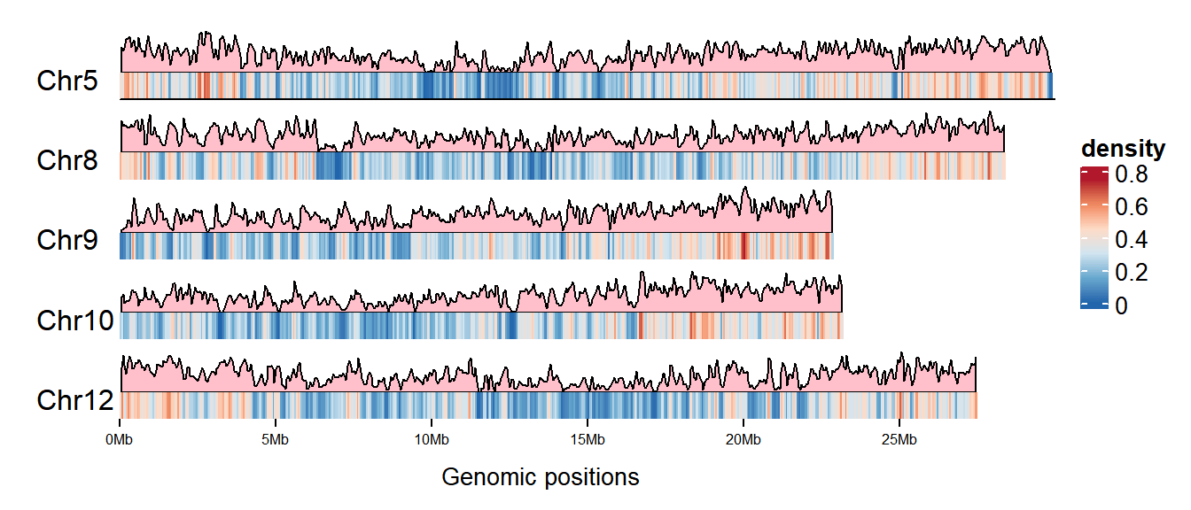
library(RColorBrewer)

Data Preparation

# Load data
data1 <- read.delim("files/Hiplot/060-gene-density-data1.txt", header = T)
data2 <- read.delim("files/Hiplot/060-gene-density-data2.txt", header = T)

# Convert data structure
chrNum <- str_replace(unique(data1$chr), "Chr|chr", "")
data1$chr <- factor(data1$chr, levels = paste0("Chr", chrNum))
data2$chr <- factor(data2$chr, levels = paste0("Chr", chrNum))
# Set window to calculate gene density
windows <- 100 * 1000 # default:100kb window size
gene_density <- genomicDensity(data2, window.size = windows)
gene_density$chr <- factor(gene_density$chr,
  levels =  paste0("Chr", chrNum)
)

# View data
head(data1)

    chr start      end
1  Chr5     0 29958434
2  Chr8     0 28443022
3  Chr9     0 23012720
4 Chr10     0 23207287
5 Chr12     0 27531856

head(data2)

    chr start   end
1 Chr10 38648 40060
2 Chr10 45941 58338
3 Chr10 67119 72971
4 Chr10 75410 76305
5 Chr10 80964 82250
6 Chr10 94798 97746

Visualization

# Set the palettes
palettes <- c("#B2182B","#EF8A62","#FDDBC7","#D1E5F0","#67A9CF","#2166AC")
col_fun <- colorRamp2(
  seq(0, max(gene_density[[4]]), length = 6), rev(palettes)
  )
cm <- ColorMapping(col_fun = col_fun)
# Set the Legend
lgd <- color_mapping_legend(
  cm, plot = F, title = "density", color_bar = "continuous"
  )
# Plot
p <- as.ggplot(function() {
  gtrellis_layout(
    data1, n_track = 2, ncol = 1, byrow = FALSE,
    track_axis = FALSE, add_name_track = FALSE,
    xpadding = c(0.1, 0), gap = unit(1, "mm"),
    track_height = unit.c(unit(1, "null"), unit(4, "mm")),
    track_ylim = c(0, max(gene_density[[4]]), 0, 1),
    border = FALSE, asist_ticks = FALSE,
    legend = lgd
    )
  # Add gene area map track
  add_lines_track(gene_density, gene_density[[4]],
                  area = TRUE, gp = gpar(fill = "pink"))
  # Add gene density heatmap track
  add_heatmap_track(gene_density, gene_density[[4]], fill = col_fun)
  add_track(track = 2, clip = FALSE, panel_fun = function(gr) {
    chr <- get_cell_meta_data("name")
    if (chr == paste("Chr", length(chrNum), sep = "")) {
      grid.lines(get_cell_meta_data("xlim"), unit(c(0, 0), "npc"),
                 default.units = "native")
      }
    grid.text(chr, x = 0.01, y = 0.38, just = c("left", "bottom"))
    })
  circos.clear()
  })

p

Figure 1: Gene Density