ggwordcloud

Authors

[Editor] Hu Zheng;

[Contributors]

Note

Hiplot website

This page is the tutorial for source code version of the Hiplot ggwordcloud plugin. You can also use the Hiplot website to achieve no code ploting. For more information please see the following link:

https://hiplot.cn/basic/ggwordcloud?lang=en

The word cloud is to visualize the “keywords” that appear frequently in the web text by forming a “keyword cloud layer” or “keyword rendering”.

Setup

System Requirements: Cross-platform (Linux/MacOS/Windows)
Programming language: R
Dependent packages: ggwordcloud

# Install packages
if (!requireNamespace("ggwordcloud", quietly = TRUE)) {
  install.packages("ggwordcloud")
}

# Load packages
library(ggwordcloud)

Data Preparation

Load data nouns and noun frequencies.

# Load data
data <- read.delim("files/Hiplot/076-ggwordcloud-data.txt", header = T)
inmask <- "files/Hiplot/076-ggwordcloud-hearth.png"

# Convert data structure
col <- data[, 2]
data <- cbind(data, col)

# View data
head(data)

    word freq col
1    oil   85  85
2   said   73  73
3 prices   48  48
4   opec   42  42
5    mln   31  31
6    the   26  26

Visualization

# ggwordcloud
p <- ggplot(data, aes(label = word, size = freq, color = col)) +
  scale_size_area(max_size = 40) +
  theme_minimal() + 
  geom_text_wordcloud_area(mask = png::readPNG(inmask), rm_outside = TRUE) +
  scale_color_gradient(low = "#8B0000", high = "#FF0000")

p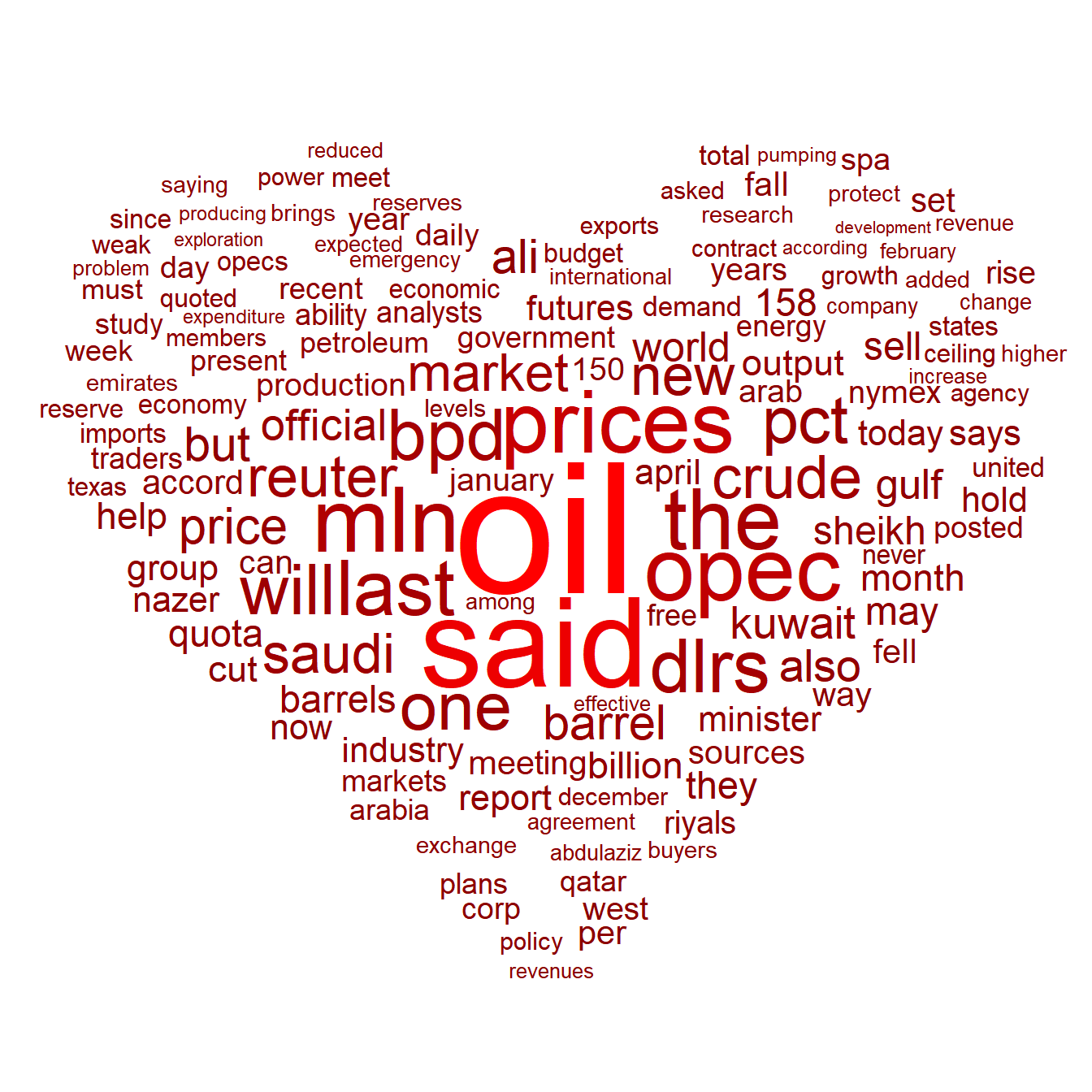

Display the proportion of nouns in the word cloud graph according to the frequency of nouns.