Chord Plot

Authors

[Editor] Hu Zheng;

[Contributors]

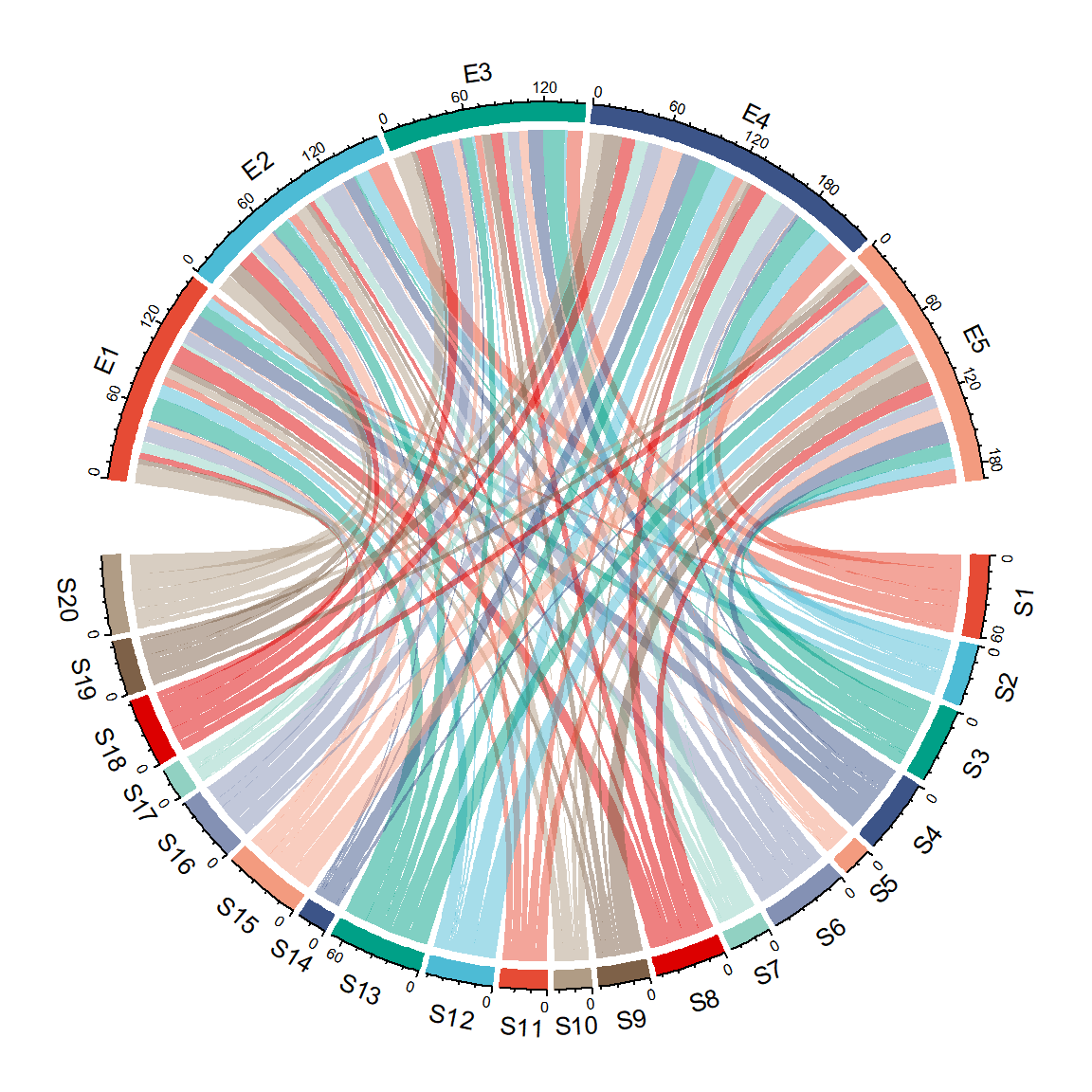
The complex interaction is visualized in the form of chord graph.

Setup

System Requirements: Cross-platform (Linux/MacOS/Windows)
Programming language: R
Dependent packages: circlize; ggplotify

# Install packages
if (!requireNamespace("circlize", quietly = TRUE)) {
  install.packages("circlize")
}
if (!requireNamespace("ggplotify", quietly = TRUE)) {
  install.packages("ggplotify")
}

# Load packages
library(circlize)
library(ggplotify)

Data Preparation

Data frame or matrix of interaction of genes with pathways or gene ontologys.

# Load data
data <- read.table("files/Hiplot/020-chord-data.txt", header = T)

# convert data structure
row.names(data) <- data[, 1]
data <- data[, -1]
data <- as.matrix(data)

# View data
head(data)

   E1 E2 E3 E4 E5
S1  4 16 12 18 11
S2  7 11  2 15 10
S3  9  2 17 16 11
S4 14  9 12  3 17
S5  1  1  7  1 12
S6 10 18  9 13  9

Visualization

# Chord Plot
Palette <- c("#E64B35FF","#4DBBD5FF","#00A087FF","#3C5488FF","#F39B7FFF",
             "#8491B4FF","#91D1C2FF","#DC0000FF","#7E6148FF","#B09C85FF")
grid.col <- c(Palette, Palette, Palette[1:5])
p <- as.ggplot(function() {
  chordDiagram(
    data, grid.col = grid.col, grid.border = NULL, transparency = 0.5,
    row.col = NULL, column.col = NULL,  order = NULL,
    directional = 0, # 1, -1, 0, 2
    direction.type = "diffHeight", # diffHeight and arrows
    diffHeight = convert_height(2, "mm"), reduce = 1e-5, xmax = NULL, 
    self.link = 2, symmetric = FALSE, keep.diagonal = FALSE, 
    preAllocateTracks = NULL,
    annotationTrack = c("name", "grid", "axis"),
    annotationTrackHeight = convert_height(c(3, 3), "mm"),
    link.border = NA, link.lwd = par("lwd"), link.lty = par("lty"), 
    link.sort = FALSE, link.decreasing = TRUE, link.largest.ontop = FALSE,
    link.visible = T, link.rank = NULL, link.overlap = FALSE,
    scale = F, group = NULL, big.gap = 10, small.gap = 1
    )
  })

p