Connected Scatterplot

Connected scatterplot

Setup

• System Requirements: Cross-platform (Linux/MacOS/Windows)

• Programming language: R

• Dependent packages: ggplot2; dplyr; ggrepel

# Install packages
if (!requireNamespace("ggplot2", quietly = TRUE)) {
  install.packages("ggplot2")
}
if (!requireNamespace("dplyr", quietly = TRUE)) {
  install.packages("dplyr")
}
if (!requireNamespace("ggrepel", quietly = TRUE)) {
  install.packages("ggrepel")
}

# Load packages
library(ggplot2)
library(dplyr)
library(ggrepel)

Data Preparation

# Load data
data <- read.table("files/Hiplot/026-connected-scatterplot-data.txt", header = T)

# View data
head(data)

  year Alice Anna
1 1991   724 7118
2 1992   686 6846
3 1993   684 6808
4 1994   595 7523
5 1995   579 8564
6 1996   593 8565

Visualization

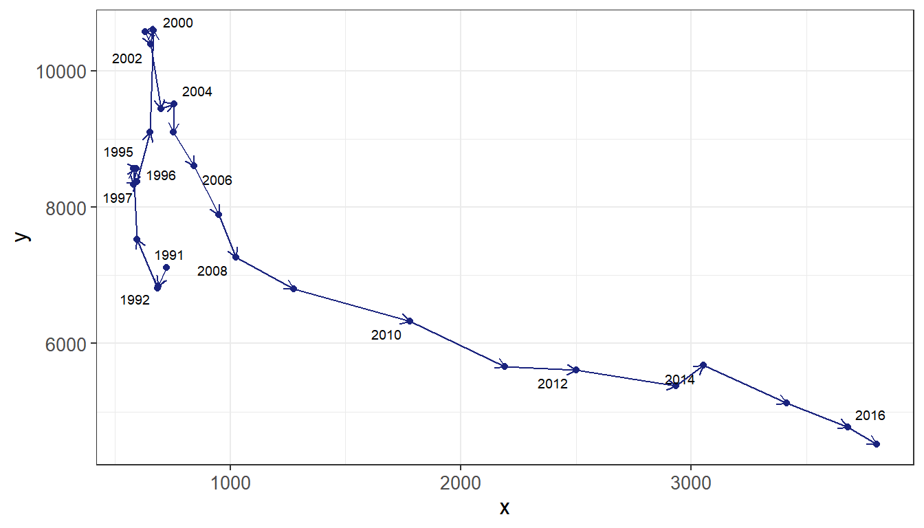
# Connected Scatterplot
connected_scatterplot <- function(data, x, y, label, label_ratio, line_color, arrow_size, label_size) {

  draw_data <- data.frame(
    x = data[[x]],
    y = data[[y]],
    label = data[[label]]
  )

  add_label_data <- draw_data %>% sample_frac(label_ratio)
  rm(data)

  p <- ggplot(draw_data, aes(x = x, y = y, label = label)) +
    geom_point(color = line_color) +
    geom_text_repel(data = add_label_data, size = label_size) +
    geom_segment(
      color = line_color,
      aes(
        xend = c(tail(x, n = -1), NA),
        yend = c(tail(y, n = -1), NA)
      ),
      arrow = arrow(length = unit(arrow_size, "mm"))
    )

  return(p)
}

p <- connected_scatterplot(
  data = if (exists("data") && is.data.frame(data)) data else "",
  x = "Alice",
  y = "Anna",
  label = "year",
  label_ratio = 0.5,
  line_color = "#1A237E",
  arrow_size = 2,
  label_size = 2.5
) +
  theme_bw() +
  theme(text = element_text(family = "Arial"),
        plot.title = element_text(size = 12,hjust = 0.5),
        axis.title = element_text(size = 12),
        axis.text = element_text(size = 10),
        axis.text.x = element_text(angle = 0, hjust = 0.5,vjust = 1),
        legend.position = "right",
        legend.direction = "vertical",
        legend.title = element_text(size = 10),
        legend.text = element_text(size = 10))

p

Figure 1: Connected Scatterplot