# Install packages
if (!requireNamespace("destiny", quietly = TRUE)) {
  install_github("theislab/destiny")
}
if (!requireNamespace("ggplotify", quietly = TRUE)) {
  install.packages("ggplotify")
}
if (!requireNamespace("scatterplot3d", quietly = TRUE)) {
  install.packages("scatterplot3d")
}
if (!requireNamespace("ggpubr", quietly = TRUE)) {
  install.packages("ggpubr")
}

# Load packages
library(destiny)
library(ggplotify)
library(scatterplot3d)
library(ggpubr)Diffusion Map
Note
Hiplot website
This page is the tutorial for source code version of the Hiplot Diffusion Map plugin. You can also use the Hiplot website to achieve no code ploting. For more information please see the following link:
Diffusion Map is a nonlinear dimensionality reduction algorithm that can be used to visualize developmental trajectories.
Setup
System Requirements: Cross-platform (Linux/MacOS/Windows)
Programming language: R
Dependent packages:
destiny;ggplotify;scatterplot3d;ggpubr
Data Preparation
# Load data
data1 <- read.delim("files/Hiplot/042-diffusion-map-data1.txt", header = T)
data2 <- read.delim("files/Hiplot/042-diffusion-map-data2.txt", header = T)

# convert data structure
sample.info <- data2
rownames(data1) <- data1[, 1]
data1 <- as.matrix(data1[, -1])
## tsne
set.seed(123)
dm_info <- DiffusionMap(t(data1))
dm_info <- cbind(DC1 = dm_info$DC1, DC2 = dm_info$DC2, DC3 = dm_info$DC3)
dm_data <- data.frame(
  sample = colnames(data1),
  dm_info
)

colorBy <- sample.info[match(colnames(data1), sample.info[, 1]), "Group"]
colorBy <- factor(colorBy, level = colorBy[!duplicated(colorBy)])
dm_data$colorBy = colorBy

# View data
head(dm_data)
sample DC1 DC2 DC3 colorBy
M1 M1 0.05059918 0.15203860 -0.06533168 G1
M2 M2 0.05030863 0.14435034 -0.06044277 G1
M3 M3 0.04271398 0.09273382 -0.02730427 G1
M4 M4 0.04680742 0.10425273 -0.03789962 G1
M5 M5 0.04971521 0.12786900 -0.05608321 G1
M6 M6 0.04840072 0.12728303 -0.05256815 G1Visualization
1. 2D
# 2D Diffusion Map
p <- ggscatter(data = dm_data,  x = "DC1", y = "DC2", color = "colorBy",
               size = 2, palette = "lancet", alpha = 1) +
  labs(color = "Group") +
  ggtitle("Diffusion Map") +
  scale_color_manual(values = c("#3B4992FF","#EE0000FF","#008B45FF")) +
  theme_classic() +
  theme(text = element_text(family = "Arial"),
        plot.title = element_text(size = 12,hjust = 0.5),
        axis.title = element_text(size = 12),
        axis.text = element_text(size = 10),
        axis.text.x = element_text(angle = 0, hjust = 0.5,vjust = 1),
        legend.position = "right",
        legend.direction = "vertical",
        legend.title = element_text(size = 10),
        legend.text = element_text(size = 10))

p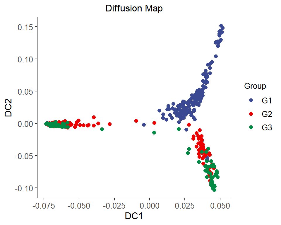
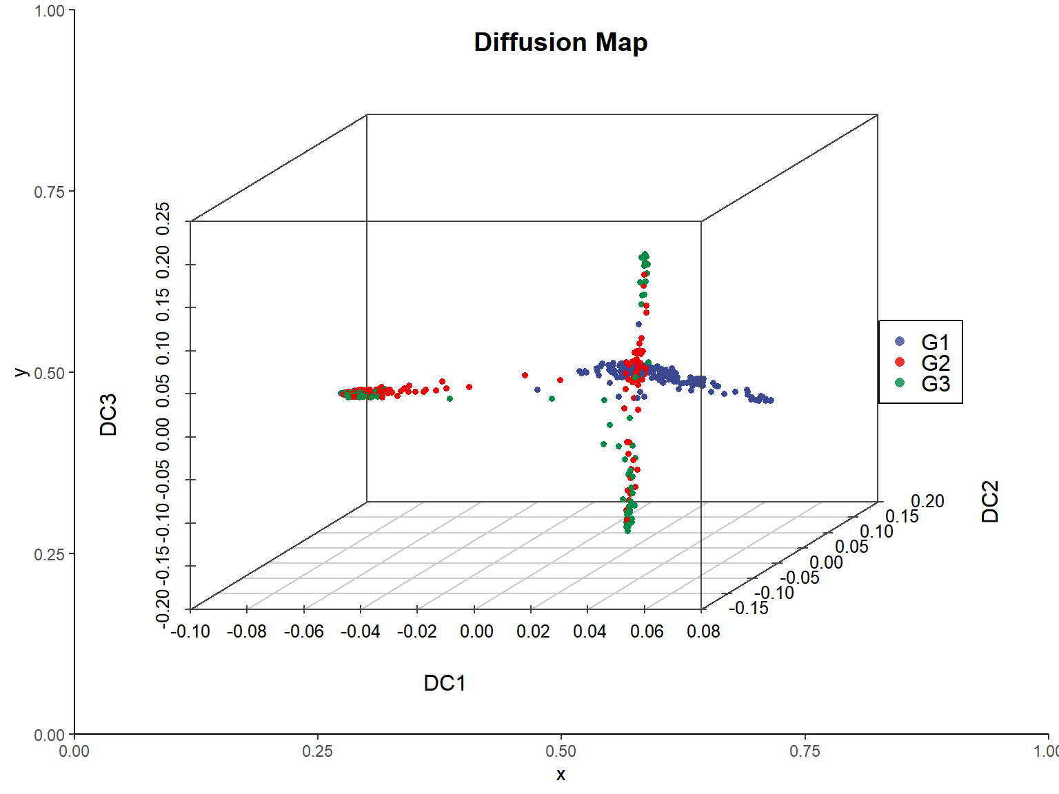
2. 3D
# 3D Diffusion Map
group.color <- c("#3B4992FF","#EE0000FF","#008B45FF")
names(group.color) <- unique(dm_data$colorBy)
group.color <- group.color[!is.na(names(group.color))]
if (length(group.color) == 0) {
  group.color <- c(Default="black")
  dm_data$colorBy <- "Default"
}
p <- as.ggplot(function(){
  scatterplot3d(x = dm_data$DC1, y = dm_data$DC2, z = dm_data$DC3,
                color =  alpha(group.color[dm_data$colorBy], 1),
                xlim=c(min(dm_data$DC1), max(dm_data$DC1)),
                ylim=c(min(dm_data$DC2), max(dm_data$DC2)),
                zlim=c(min(dm_data$DC3), max(dm_data$DC3)),
                pch = 16, cex.symbols  = 0.6,
                scale.y = 0.8,
                xlab = "DC1", ylab = "DC2", zlab = "DC3",
                angle = 40,
                main = "Diffusion Map",
                col.axis = "#444444", col.grid = "#CCCCCC")
  legend("right", legend = names(group.color),
         col = alpha(group.color, 0.8), pch = 16)
    })
p <- p + theme_classic()

p