Gene Cluster Trend

The gene cluster trend is used to display different gene expression trend with multiple lines showing the similar expression patterns in each cluster.

Setup

• System Requirements: Cross-platform (Linux/MacOS/Windows)

• Programming language: R

• Dependent packages: Mfuzz; ggplotify; RColorBrewer

# Install packages
if (!requireNamespace("Mfuzz", quietly = TRUE)) {
  install_github("MatthiasFutschik/Mfuzz")
}
if (!requireNamespace("ggplotify", quietly = TRUE)) {
  install.packages("ggplotify")
}
if (!requireNamespace("RColorBrewer", quietly = TRUE)) {
  install.packages("RColorBrewer")
}

# Load packages
library(Mfuzz)
library(ggplotify)
library(RColorBrewer)

Data Preparation

The loaded data are a gene expression matrix with each row represent a gene and each column represent a time-point sample.

# Load data
data <- read.delim("files/Hiplot/062-gene-trend-data.txt", header = T)

# Convert data structure
## Convert a gene expression matrix to an ExpressionSet object
row.names(data) <- data[,1]
data <- data[,-1]
data <- as.matrix(data)
eset <- new("ExpressionSet", exprs = data)
## Filter genes with more than 25% missing values
eset <- filter.NA(eset, thres=0.25)

0 genes excluded.

## Remove genes with small differences between samples based on standard deviation
eset <- filter.std(eset, min.std=0, visu = F)

0 genes excluded.

## Data Standardization
eset <- standardise(eset)
## Set the number of clusters
c <- 6
## Evaluate the optimal m value
m <- mestimate(eset)
## Perform mfuzz clustering
cl <- mfuzz(eset, c = c, m = m)

# View data
head(data)

           Time1      Time2       Time3
Gene1  0.1774993  1.6563226 -1.15259948
Gene2 -0.5037254 -0.5207024  0.46416071
Gene3  0.1050310  0.6079246  0.72893247
Gene4 -1.1791537  0.4340085  0.41061745
Gene5  0.8368975 -0.7047414 -1.46114720
Gene6  0.2611762  0.1351524 -0.01890809

Visualization

# Gene Cluster Trend
p <- as.ggplot(function(){
  mfuzz.plot2(
  eset,
  cl,
  xlab = "Time",
  ylab = "Expression changes",
  mfrow = c(2,(c/2+0.5)),
  colo = "fancy",
  centre = T,
  centre.col = "red",
  time.labels = colnames(eset),
  x11=F)
  })

p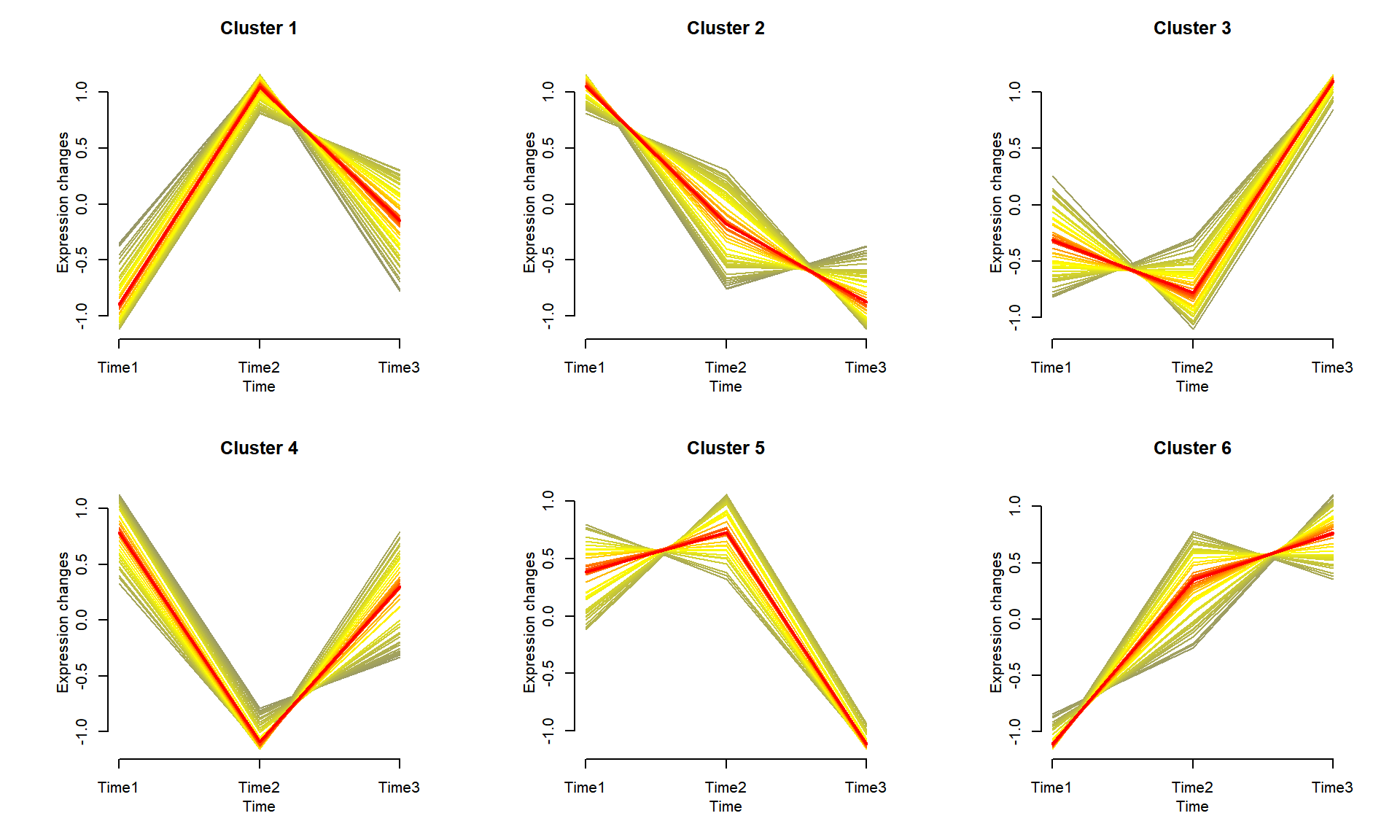

Figure 1: Gene Cluster Trend

As shown in the example figure, the genes are clustered into different groups, with each group showing similar expression patterns across different time-points. The average expression trend is highlighted in each cluster.