Diverging Scale

Authors

[Editor] Hu Zheng;

[Contributors]

The diverging scale is a graph that maps a continuous, quantitative input to a continuous fixed interpolator.

Setup

System Requirements: Cross-platform (Linux/MacOS/Windows)
Programming language: R
Dependent packages: ggcharts

# Install packages
if (!requireNamespace("ggcharts", quietly = TRUE)) {
  install.packages("ggcharts")
}

# Load packages
library(ggcharts)

Data Preparation

The first column is a list of model names, and the remaining columns enter the relevant indicators and corresponding values.

# Load data
data <- read.delim("files/Hiplot/043-diverging-scale-data.txt", header = T)

# convert data structure
data <- dplyr::transmute(.data = data, x = model, y = scale(hp))

# View data
head(data)

                  x          y
1         Mazda RX4 -0.6130929
2     Mazda RX4 Wag -0.6130929
3        Datsun 710 -0.9123057
4    Hornet 4 Drive -0.6130929
5 Hornet Sportabout  0.5309561
6           Valiant -0.7010967

Visualization

1.Barplot

# Diverging Scale Barplot
fill_colors <- c("#C20B01", "#196ABD")
fill_colors <- fill_colors[c(any(data[, "y"] > 0), any(data[, "y"] < 0))]
p <- diverging_bar_chart(data = data, x = x, y = y, bar_colors = fill_colors,
                         text_color = '#000000') + 
  theme(axis.text.x = element_text(color = "#000000"),
        axis.title.x = element_text(colour = "#000000"),
        axis.title.y = element_text(colour = "#000000"),
        plot.background = element_blank()) + 
  labs(x = "model", y = "scale(hp)", title = "")

p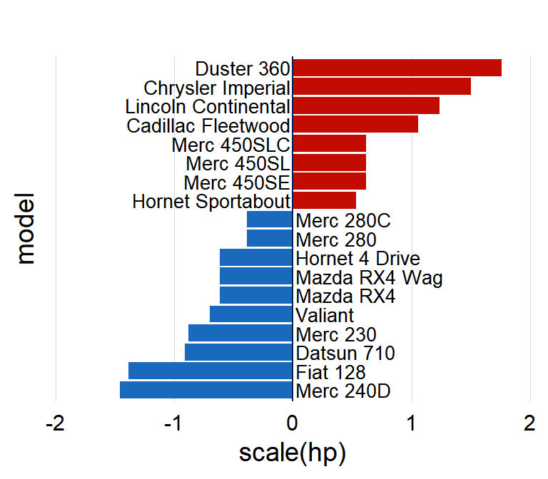

Hp data is shown on the horizontal axis, model names (classification) are shown on the vertical axis, models above average are shown in red, and models below average are shown in blue. Data is assigned on a scale of 2 by size.

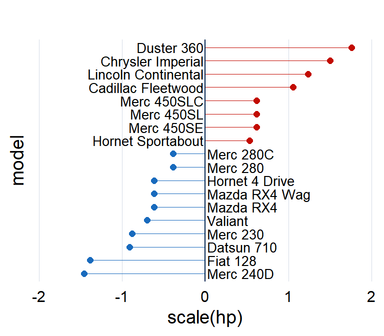
2.Lollipop Plot

# Diverging Scale Lollipop Plot
fill_colors <- c("#C20B01", "#196ABD")
fill_colors <- fill_colors[c(any(data[, "y"] > 0), any(data[, "y"] < 0))]
p <- diverging_lollipop_chart(
  data = data, x = x, y = y, lollipop_colors = fill_colors,
  line_size = 0.3, point_size = 1.9, text_color = '#000000') + 
  theme(axis.text.x = element_text(color = "#000000"),
        axis.title.x = element_text(colour = "#000000"),
        axis.title.y = element_text(colour = "#000000"),
        plot.background = element_blank()) + 
  labs(x = "model", y = "scale(hp)", title = "")

p