DIY GSEA

Authors

[Editor] Hu Zheng;

[Contributors]

Note

Hiplot website

This page is the tutorial for source code version of the Hiplot DIY GSEA plugin. You can also use the Hiplot website to achieve no code ploting. For more information please see the following link:

https://hiplot.cn/basic/diy-gsea?lang=en

Make your geneset.

Setup

System Requirements: Cross-platform (Linux/MacOS/Windows)
Programming language: R
Dependent packages: clusterProfiler

# Install packages
if (!requireNamespace("clusterProfiler", quietly = TRUE)) {
  install_github("YuLab-SMU/clusterProfiler")
}

# Load packages
library(clusterProfiler)

Data Preparation

# Load data
data1 <- read.delim("files/Hiplot/044-diy-gsea-data1.txt", header = T)
data2 <- read.delim("files/Hiplot/044-diy-gsea-data2.txt", header = T)

# convert data structure
data1[,2] <- as.numeric(data1[,2])
geneList <- data1[,2]
names(geneList) <- data1[,1]
geneList <- sort(geneList, decreasing = TRUE)
term <- data.frame(term=data2[,1], gene=data2[,2])

# View data
head(term)

                         term   gene
1 GO_ADAPTIVE_IMMUNE_RESPONSE ADAM17
2 GO_ADAPTIVE_IMMUNE_RESPONSE  AICDA
3 GO_ADAPTIVE_IMMUNE_RESPONSE  ALCAM
4 GO_ADAPTIVE_IMMUNE_RESPONSE  ANXA1
5 GO_ADAPTIVE_IMMUNE_RESPONSE   BATF
6 GO_ADAPTIVE_IMMUNE_RESPONSE  BCL10

Visualization

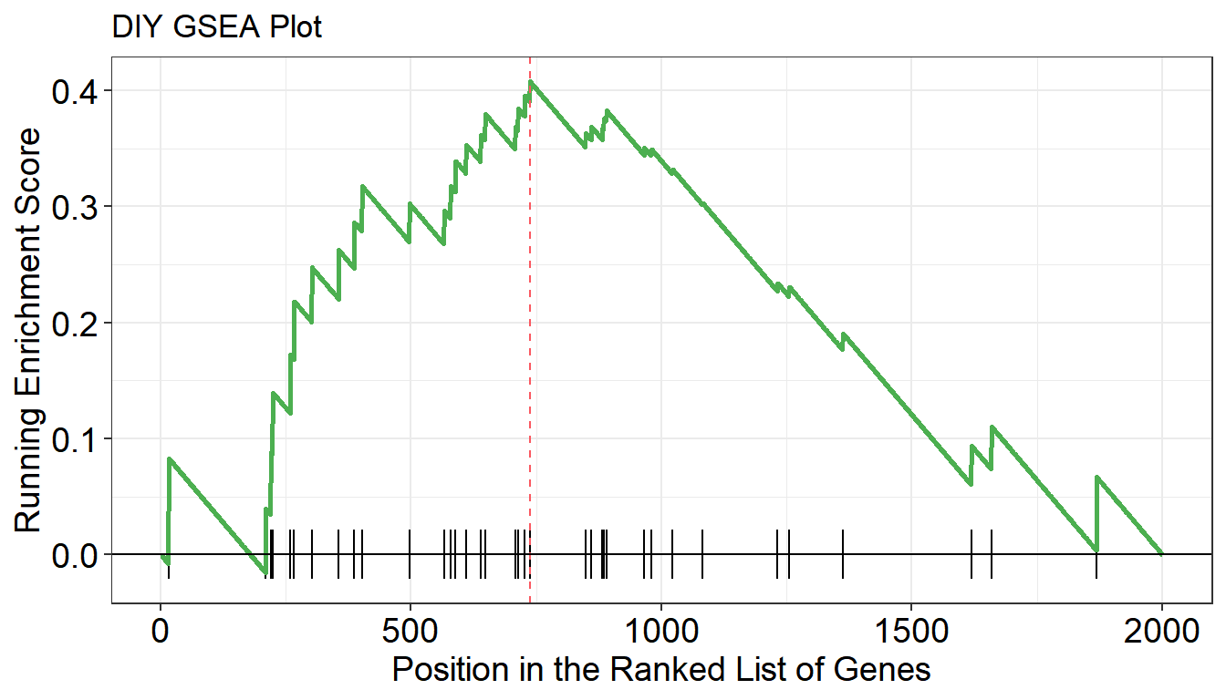
# DIY GSEA
y <- clusterProfiler::GSEA(geneList, TERM2GENE = term, pvalueCutoff = 1)
p <- gseaplot(
  y,
  y@result$Description[1],
  color = "#000000",
  by = "runningScore",
  color.line = "#4CAF50",
  color.vline= "#FA5860",
  title = "DIY GSEA Plot",
  )

p