世界地图

作者

[编辑] 郑虎;

[审核] .

注记

Hiplot 网站

本页面为 Hiplot World Map 插件的源码版本教程，您也可以使用 Hiplot 网站实现无代码绘图，更多信息请查看以下链接:

https://hiplot.cn/basic/map-world?lang=zh_cn

环境配置

系统: Cross-platform (Linux/MacOS/Windows)
编程语言: R
依赖包: ggplot2; RColorBrewer

# 安装包
if (!requireNamespace("ggplot2", quietly = TRUE)) {
  install.packages("ggplot2")
}
if (!requireNamespace("RColorBrewer", quietly = TRUE)) {
  install.packages("RColorBrewer")
}

# 加载包
library(ggplot2)
library(RColorBrewer)

数据准备

# 加载数据
data <- read.delim("files/Hiplot/116-map-world-data.txt", header = T)
dt_map <- readRDS("files/Hiplot/world.rds")

# 整理数据格式
dt_map$Value <- data$death_rate[match(dt_map$ENG_NAME, data$region)]

# 查看数据
head(data)

          region death_rate
1    Afghanistan       13.4
2        Albania        6.8
3        Algeria        4.3
4 American Samoa        5.9
5        Andorra        7.3
6         Angola        9.2

可视化

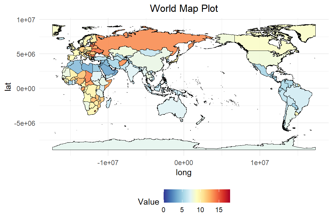
# 世界地图
p <- ggplot(dt_map) +
  geom_polygon(aes(x = long, y = lat, group = group, fill = Value),
               alpha = 0.9, size = 0.5) +
  geom_path(aes(x = long, y = lat, group = group), 
            color = "black", size = 0.2) +
  scale_fill_gradientn(
    colours = colorRampPalette(rev(brewer.pal(11,"RdYlBu")))(500),
    na.value = "grey10",
    limits = c(0, max(dt_map$Value) * 1.2)) +
    ggtitle("World Map Plot") +
  theme_minimal() +
  theme(plot.title = element_text(hjust = 0.5),
        legend.position = "bottom", legend.direction = "horizontal")

p