斜面图

作者

[编辑] 郑虎;

[审核] .

注记

Hiplot 网站

本页面为 Hiplot Slopegraph 插件的源码版本教程，您也可以使用 Hiplot 网站实现无代码绘图，更多信息请查看以下链接:

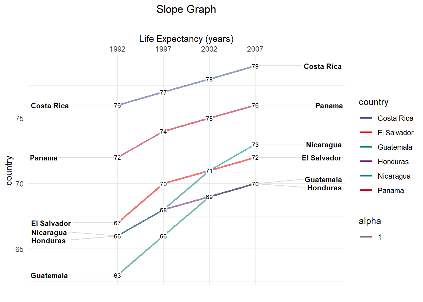
https://hiplot.cn/basic/slopegraph?lang=zh_cn

斜面图可以用于展示数值变化情况。

环境配置

系统: Cross-platform (Linux/MacOS/Windows)
编程语言: R
依赖包: CGPfunctions; ggplot2

# 安装包
if (!requireNamespace("CGPfunctions", quietly = TRUE)) {
  install.packages("CGPfunctions")
}
if (!requireNamespace("ggplot2", quietly = TRUE)) {
  install.packages("ggplot2")
}

# 加载包
library(CGPfunctions)
library(ggplot2)

数据准备

# 加载数据
data <- read.delim("files/Hiplot/165-slopegraph-data.txt", header = T)

# 整理数据格式
data[, "country"] <- factor(data[ ,"country"], levels = unique(data[ ,"country"]))
data[, "year"] <- factor(data[ ,"year"], levels = unique(data[ ,"year"]))

# 查看数据
head(data)

      country continent year lifeExp     pop gdpPercap
1  Costa Rica  Americas 1992      76 3173216  6160.416
2  Costa Rica  Americas 1997      77 3518107  6677.045
3  Costa Rica  Americas 2002      78 3834934  7723.447
4  Costa Rica  Americas 2007      79 4133884  9645.061
5 El Salvador  Americas 1992      67 5274649  4444.232
6 El Salvador  Americas 1997      70 5783439  5154.825

可视化

# 斜面图
p <- newggslopegraph(data, year, lifeExp, country) +
  labs(subtitle = "", title = "Slope Graph", x = "Life Expectancy (years)",
       y = "country", caption = "") +
  scale_color_manual(values = c("#3B4992FF", "#EE0000FF", "#008B45FF",
                               "#631879FF", "#008280FF", "#BB0021FF")) +
  theme_minimal() +
  theme(plot.title = element_text(hjust = 0.5))

p