# 安装包
if (!requireNamespace("ggplot2", quietly = TRUE)) {
  install.packages("ggplot2")
}
if (!requireNamespace("ggthemes", quietly = TRUE)) {
  install.packages("ggthemes")
}

# 加载包
library(ggplot2)
library(ggthemes)丝带图
注记
Hiplot 网站
本页面为 Hiplot Ribbon 插件的源码版本教程,您也可以使用 Hiplot 网站实现无代码绘图,更多信息请查看以下链接:
丝带图是一种类似丝带的图形。
环境配置
系统: Cross-platform (Linux/MacOS/Windows)
编程语言: R
依赖包:
ggplot2;ggthemes
数据准备
载入数据为 x 轴数值及其对应的两个 y 轴数值和分组。
# 加载数据
data <- read.delim("files/Hiplot/153-ribbon-data.txt", header = T)

# 整理数据格式
colnames(data) <- c("group", "xvalue", "yvalue1", "yvalue2")
data$yvalue <- (data$yvalue1 + data$yvalue2) / 2

# 查看数据
head(data)
group xvalue yvalue1 yvalue2 yvalue
1 Group1 1900 -0.279 -0.063 -0.171
2 Group1 1901 -0.271 -0.053 -0.162
3 Group1 1902 -0.285 -0.069 -0.177
4 Group1 1903 -0.303 -0.095 -0.199
5 Group1 1904 -0.328 -0.118 -0.223
6 Group1 1905 -0.348 -0.134 -0.241可视化
# 丝带图
p <- ggplot(data, aes(xvalue, yvalue, fill = group)) +
  geom_ribbon(alpha = 0.2, aes(ymin = yvalue1, ymax = yvalue2)) +
  geom_line(aes(y = yvalue, color = group), lwd = 1) +
  geom_line(aes(y = yvalue1, color = group), linetype = "dotted") +
  geom_line(aes(y = yvalue2, color = group), linetype = "dotted") +
  ylab("y axis value") +
  xlab("x axis value") +
  ggtitle("Ribbon Plot") +
  scale_fill_manual(values = c("#e04d39","#5bbad6")) +
  scale_color_manual(values = c("#e04d39","#5bbad6")) +
  theme_stata() +
  theme(text = element_text(family = "Arial"),
        plot.title = element_text(size = 12,hjust = 0.5),
        axis.title = element_text(size = 12),
        axis.text = element_text(size = 10),
        axis.text.x = element_text(angle = 0, hjust = 0.5,vjust = 1),
        legend.position = "right",
        legend.direction = "vertical",
        legend.title = element_text(size = 10),
        legend.text = element_text(size = 10))

p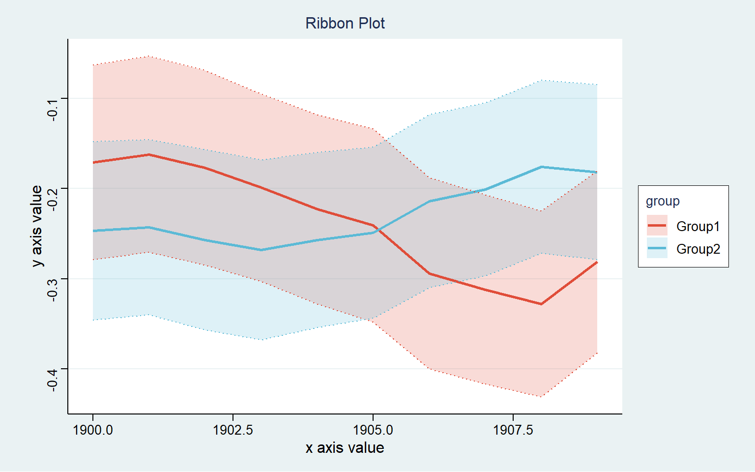
每种颜色表示不同的分组,可以透过其中折线,观测每组数据随时间的变化。