# 安装包
if (!requireNamespace("Rtsne", quietly = TRUE)) {
  install.packages("Rtsne")
}
if (!requireNamespace("ggpubr", quietly = TRUE)) {
  install.packages("ggpubr")
}

# 加载包
library(Rtsne)
library(ggpubr)tSNE
注记
Hiplot 网站
本页面为 Hiplot tSNE 插件的源码版本教程,您也可以使用 Hiplot 网站实现无代码绘图,更多信息请查看以下链接:
t-SNE 是一种非线性降维算法,适用于高维数据降维到 2 维或 3 维并进行可视化。该算法能够使较大相似度的点,t 分布在低维空间中的距离更近;而对于低相似度的点,t 分布在低维空间中的距离更远。
环境配置
系统: Cross-platform (Linux/MacOS/Windows)
编程语言: R
依赖包:
Rtsne;ggpubr
数据准备
载入数据为数据集(基因名称及其对应的基因表达值)和样本信息(样本名称及分组)。
# 加载数据
data1 <- read.delim("files/Hiplot/175-tsne-data1.txt", header = T)
data2 <- read.delim("files/Hiplot/175-tsne-data2.txt", header = T)

# 整理数据格式
sample.info <- data2
rownames(data1) <- data1[, 1]
data1 <- as.matrix(data1[, -1])
## tsne
set.seed(123)
tsne_info <- Rtsne(t(data1), perplexity = 1, theta = 0.1, check_duplicates = FALSE)
colnames(tsne_info$Y) <- c("tSNE_1", "tSNE_2")
# handle data
tsne_data <- data.frame(
  sample = colnames(data1),
  tsne_info$Y
)
colorBy <- sample.info[match(colnames(data1), sample.info[, 1]), "group"]
colorBy <- factor(colorBy, level = colorBy[!duplicated(colorBy)])
tsne_data$colorBy = colorBy
shapeBy <- NULL

# 查看数据
head(data1)
M1 M2 M3 M8 M9 M10
GBP4 6.599344 5.226266 3.693288 7.658312 8.666038 7.419708
BCAT1 5.760380 4.892783 5.448924 8.765915 8.097206 8.262942
CMPK2 9.561905 4.549168 3.998655 7.379591 7.938063 6.154118
STOX2 8.396409 8.717055 8.039064 3.542217 4.305187 6.964710
PADI2 8.419766 8.268430 8.451181 4.136667 4.910986 4.080363
SCARNA5 7.653074 5.780393 10.633550 3.822596 4.041078 7.956589head(data2) sample group
1 M1 G1
2 M2 G1
3 M3 G1
4 M8 G2
5 M9 G2
6 M10 G2可视化
# tsne
p <- ggscatter(data = tsne_data, x = "tSNE_1", y = "tSNE_2", size = 2,
               palette = "lancet", color = "colorBy") +
  labs(color = "group") +
  ggtitle("tSNE Plot1") +
  theme_bw() +
  theme(text = element_text(family = "Arial"),
        plot.title = element_text(size = 12,hjust = 0.5),
        axis.title = element_text(size = 12),
        axis.text = element_text(size = 10),
        axis.text.x = element_text(angle = 0, hjust = 0.5,vjust = 1),
        legend.position = "right",
        legend.direction = "vertical",
        legend.title = element_text(size = 10),
        legend.text = element_text(size = 10))

p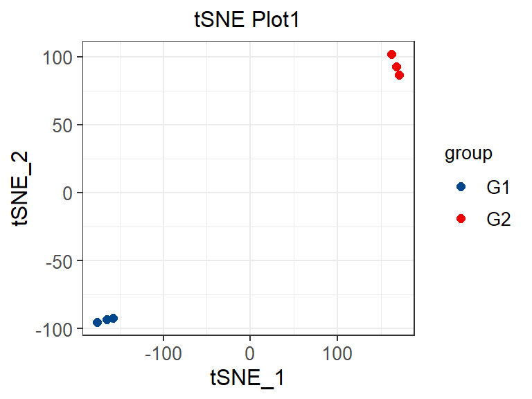
不同颜色表示不同样本,与 PCA(主成分分析)图形解释相同,不同之处在于可视化效果,t-SNE 中对于不相似的点,用一个较小的距离会产生较大的梯度来让这些点排斥开来。