# 安装包
if (!requireNamespace("PCAtools", quietly = TRUE)) {
  install_github('kevinblighe/PCAtools')
}
if (!requireNamespace("ggplotify", quietly = TRUE)) {
  install.packages("ggplotify")
}
if (!requireNamespace("cowplot", quietly = TRUE)) {
  install.packages("cowplot")
}

# 加载包
library(PCAtools)
library(ggplotify)
library(cowplot)主成分分析 (PCAtools)
注记
Hiplot 网站
本页面为 Hiplot PCAtools 插件的源码版本教程,您也可以使用 Hiplot 网站实现无代码绘图,更多信息请查看以下链接:
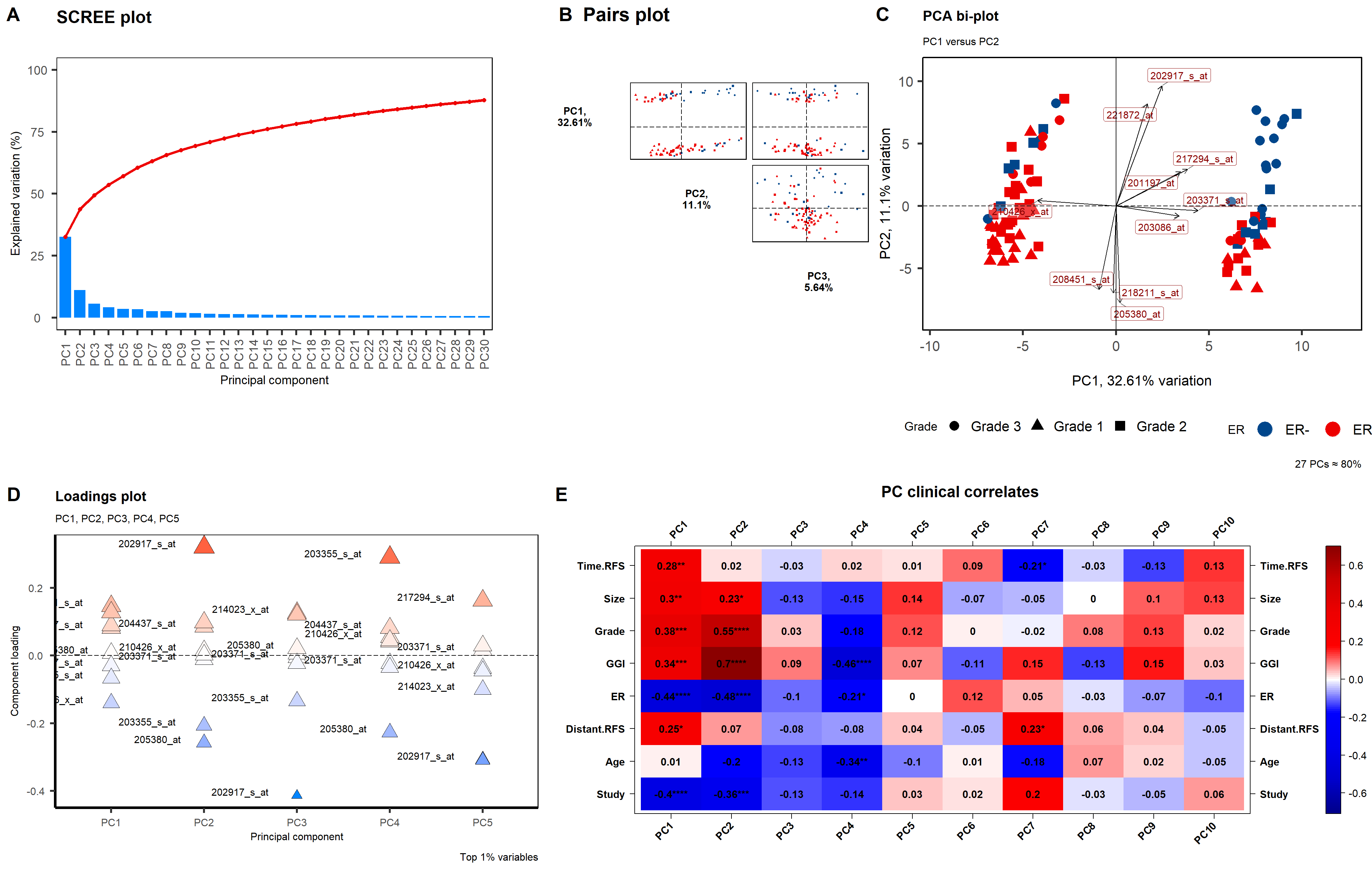
PCAtools 可以通过主成分分析对数据进行降维,并在二维水平查看主成分相关特征。
环境配置
系统: Cross-platform (Linux/MacOS/Windows)
编程语言: R
依赖包:
PCAtools;ggplotify;cowplot
数据准备
- 数据表格 1(数值矩阵):
每一列为一个样本,每一行为一个特征(如基因、芯片探针)。
- 数据表格 2 (样本信息):
第一列为样本名,其他列为该样本的表型特征,可用于标注点的颜色和形状,并与主成分进行相关性分析。
# 加载数据
data <- read.delim("files/Hiplot/136-pcatools-data1.txt", header = T)
data2 <- read.delim("files/Hiplot/136-pcatools-data2.txt", header = T)

# 查看数据
head(data[,1:5])
Probes GSM65752 GSM65753 GSM65755 GSM65757
1 220050_at 6.566843 5.902831 5.185271 5.474453
2 213944_x_at 8.722271 9.088407 9.106401 8.900869
3 215441_at 3.812778 3.852745 3.846690 3.842543
4 214792_x_at 6.499815 6.731196 5.951202 6.578830
5 217251_x_at 6.607354 6.555413 6.715821 6.628053
6 207406_at 3.997302 3.964112 3.836560 3.833057head(data2) Samplename Study Age Distant.RFS ER GGI Grade Size Time.RFS
1 GSM65752 GSE47561 40 0 ER- 2.480050 Grade 3 1.2 2280
2 GSM65753 GSE47561 46 0 ER+ -0.633592 Grade 1 1.3 2675
3 GSM65755 GSE47561 41 1 ER+ 1.043950 Grade 3 3.3 182
4 GSM65757 GSE47561 34 0 ER+ 1.059190 Grade 2 1.6 3952
5 GSM65758 GSE47561 46 1 ER+ -1.233060 Grade 2 2.1 1824
6 GSM65760 GSE47561 57 1 ER+ 0.679034 Grade 3 2.2 699可视化
# 主成分分析 (PCAtools)
## 定义绘图函数
call_pcatools <- function(datTable, sampleInfo,
                          top_var,
                          screeplotComponents, screeplotColBar,
                          pairsplotComponents,
                          biplotShapeBy, biplotColBy,
                          plotloadingsComponents,
                          plotloadingsLowCol,
                          plotloadingsMidCol,
                          plotloadingsHighCol,
                          eigencorplotMetavars,
                          eigencorplotComponents) {
  row.names(datTable) <- datTable[, 1]
  datTable <- datTable[, -1]
  row.names(sampleInfo) <- sampleInfo[, 1]
  data3 <<- pca(datTable, metadata = sampleInfo, removeVar = (100 - top_var) / 100)

  for (i in c("screeplotComponents", "pairsplotComponents",
              "plotloadingsComponents", "eigencorplotComponents")) {
    if (ncol(data3$rotated) < get(i)) {
      assign(i, ncol(data3$rotated))
    }
  }

  p1 <- PCAtools::screeplot(
    data3,
    components = getComponents(data3, 1:screeplotComponents),
    axisLabSize = 14, titleLabSize = 20,
    colBar = screeplotColBar,
    gridlines.major = FALSE, gridlines.minor = FALSE,
    returnPlot = TRUE
  )

  params_pairsplot <- list(
    data3,
    components = getComponents(data3, c(1:pairsplotComponents)),
    triangle = TRUE, trianglelabSize = 12,
    hline = 0, vline = 0,
    pointSize = 0.8, gridlines.major = FALSE, gridlines.minor = FALSE,
    title = "", plotaxes = FALSE,
    margingaps = unit(c(0.01, 0.01, 0.01, 0.01), "cm"),
    returnPlot = TRUE,
    colkey = c("#00468BFF","#ED0000FF"),
    legendPosition = "none"
  )
  params_biplot <- list(data3,
    showLoadings = TRUE,
    lengthLoadingsArrowsFactor = 1.5,
    sizeLoadingsNames = 4,
    colLoadingsNames = "red4",
    # other parameters
    lab = NULL,
    hline = 0, vline = c(-25, 0, 25),
    vlineType = c("dotdash", "solid", "dashed"),
    gridlines.major = FALSE, gridlines.minor = FALSE,
    pointSize = 5,
    legendLabSize = 16, legendIconSize = 8.0,
    drawConnectors = FALSE,
    title = "PCA bi-plot",
    subtitle = "PC1 versus PC2",
    caption = "27 PCs ≈ 80%",
    returnPlot = TRUE,
    legendPosition = "bottom"
  )
  if (!is.null(biplotShapeBy) && biplotShapeBy != "") {
    params_biplot$shape <- biplotShapeBy
    params_pairsplot$shape <- biplotShapeBy
    t <- params_biplot[[1]]$metadata[,biplotShapeBy]
    params_biplot[[1]]$metadata[,biplotShapeBy] <- factor(t,
      levels = t[!duplicated(t)]
    )
    params_pairsplot[[1]]$metadata[,biplotShapeBy] <- factor(t,
      levels = t[!duplicated(t)]
    )
  }
  if (!is.null(biplotColBy) && biplotColBy != "") {
    params_pairsplot$colby <- biplotColBy
    params_pairsplot$colkey <- c("#00468BFF","#ED0000FF")
    params_biplot$colby <- biplotColBy
    params_biplot$colkey <- c("#00468BFF","#ED0000FF")
    t1 <- params_biplot[[1]]$metadata[,biplotColBy]
    params_biplot[[1]]$metadata[,biplotColBy] <- factor(t1,
      levels = t1[!duplicated(t1)]
    )
    params_pairsplot[[1]]$metadata[,biplotColBy] <- factor(t1,
      levels = t1[!duplicated(t1)]
    )
  }

  p2 <- do.call(PCAtools::pairsplot, params_pairsplot)
  p3 <- do.call(PCAtools::biplot, params_biplot)

  p4 <- PCAtools::plotloadings(
    data3,
    rangeRetain = 0.01, labSize = 4,
    components = getComponents(data3, c(1:plotloadingsComponents)),
    title = "Loadings plot", axisLabSize = 12,
    subtitle = "PC1, PC2, PC3, PC4, PC5",
    caption = "Top 1% variables",
    gridlines.major = FALSE, gridlines.minor = FALSE,
    shape = 24, shapeSizeRange = c(4, 8),
    col = c(plotloadingsLowCol, plotloadingsMidCol, plotloadingsHighCol),
    legendPosition = "none",
    drawConnectors = FALSE,
    returnPlot = TRUE
  )

  if (length(eigencorplotMetavars) > 0 && all(eigencorplotMetavars != "")) {
    metavars <- eigencorplotMetavars
  } else {
    metavars <- colnames(sampleInfo)[2:ncol(sampleInfo)]
  }
  if (length(metavars) == 1 && metavars != colnames(sampleInfo)[1]) {
    metavars <- c(colnames(sampleInfo)[1], metavars)
  } else if (length(metavars) == 1 && metavars == colnames(sampleInfo)[1]) {
    stop('eigencorplotMetavars need >= 2 feature')
  }

  p5 <- PCAtools::eigencorplot(
    data3,
    components = getComponents(data3, 1:eigencorplotComponents),
    metavars = metavars,
    cexCorval = 1.0,
    fontCorval = 2,
    posLab = "all",
    rotLabX = 45,
    scale = TRUE,
    main = "PC clinical correlates",
    cexMain = 1.5,
    plotRsquared = FALSE,
    corFUN = "pearson",
    corUSE = "na.or.complete",
    signifSymbols = c("****", "***", "**", "*", ""),
    signifCutpoints = c(0, 0.0001, 0.001, 0.01, 0.05, 1),
    returnPlot = TRUE
  )

  p6 <- plot_grid(
    p1, p2, p3,
    ncol = 3,
    labels = c("A", "B  Pairs plot", "C"),
    label_fontfamily = "Arial",
    label_fontface = "bold",
    label_size = 22,
    align = "h",
    rel_widths = c(1.10, 0.80, 1.10)
  )

  p7 <- plot_grid(
    p4,
    as.grob(p5),
    ncol = 2,
    labels = c("D", "E"),
    label_fontfamily = "Arial",
    label_fontface = "bold",
    label_size = 22,
    align = "h",
    rel_widths = c(0.8, 1.2)
  )

  p <- plot_grid(
    p6, p7,
    ncol = 1,
    rel_heights = c(1.1, 0.9)
  )

  return(p)
}

## 绘图
p <- call_pcatools(
  datTable = data,
  sampleInfo = data2,
  biplotColBy = "ER",
  biplotShapeBy = "Grade",
  eigencorplotMetavars = colnames(data2)[-1],
  screeplotComponents = 30,
  pairsplotComponents = 3,
  plotloadingsComponents = 5,
  eigencorplotComponents = 10,
  top_var = 90,
  screeplotColBar = "#0085FF",
  plotloadingsLowCol = "#0085FF",
  plotloadingsMidCol = "#FFFFFF",
  plotloadingsHighCol = "#FF0000"
)

p