# 安装包
if (!requireNamespace("survival", quietly = TRUE)) {
  install.packages("survival")
}
if (!requireNamespace("rms", quietly = TRUE)) {
  install.packages("rms")
}
if (!requireNamespace("ggplotify", quietly = TRUE)) {
  install.packages("ggplotify")
}

# 加载包
library(survival)
library(rms)
library(ggplotify)诺莫图
注记
Hiplot 网站
本页面为 Hiplot Nomogram 插件的源码版本教程,您也可以使用 Hiplot 网站实现无代码绘图,更多信息请查看以下链接:
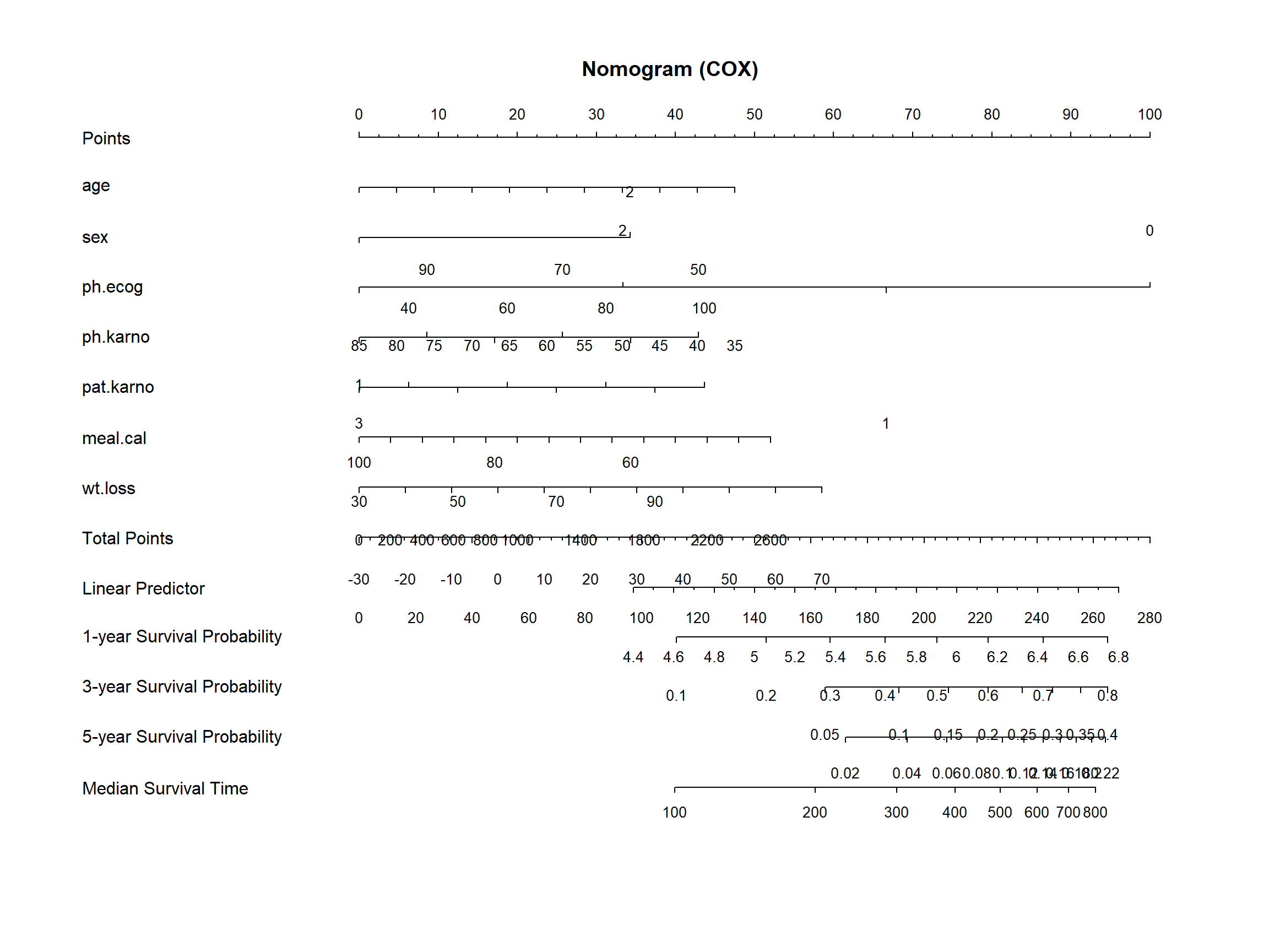
列线图常被用来评价肿瘤和医学的预后,并能直观地反映logistic回归或Cox回归的结果。
环境配置
系统: Cross-platform (Linux/MacOS/Windows)
编程语言: R
依赖包:
survival;rms;ggplotify
数据准备
随时间变化的生存数据帧,根据实例数据用0,1等数字表示性别和状态。
# 加载数据
data <- read.delim("files/Hiplot/131-nomogram-data.txt", header = T)

# 整理数据格式
dd <- datadist(data)
options(datadist = "dd")
## 建立 COX 模型并运行列线图
cox_res <- psm(
  data = data,
  as.formula(paste(
    sprintf("Surv(%s, %s) ~ ", colnames(data)[1], colnames(data)[2]),
    paste(colnames(data)[3:length(colnames(data))],
      collapse = "+"
    )
  )),
  # Surv(time, status) ~ age + sex + ph.ecog + ph.karno + pat.karno,
  dist = "lognormal"
)
## 建立 Survival 概率函数
surv <- Survival(cox_res)
## 构建分位数生存时间函数
med <- Quantile(cox_res)

cox_nomo <- nomogram(
  cox_res,
  fun = list(function(x) surv(365, x), function(x) surv(1095, x),
             function(x) surv(1825, x), function(x) med(lp = x)),
  funlabel = c("1-year Survival Probability",
               "3-year Survival Probability",
               "5-year Survival Probability",
               "Median Survival Time"),
  maxscale = 100
)

# 查看数据
head(data)
time status age sex ph.ecog ph.karno pat.karno meal.cal wt.loss
1 306 2 74 1 1 90 100 1175 NA
2 455 2 68 1 0 90 90 1225 15
3 1010 1 56 1 0 90 90 NA 15
4 210 2 57 1 1 90 60 1150 11
5 883 2 60 1 0 100 90 NA 0
6 1022 1 74 1 1 50 80 513 0可视化
# 诺莫图
p <- as.ggplot(function() {
  plot(cox_nomo, scale = 1)
  title(main = "Nomogram (COX)")
})

p