# 安装包
if (!requireNamespace("plotROC", quietly = TRUE)) {
  install.packages("plotROC")
}
if (!requireNamespace("survivalROC", quietly = TRUE)) {
  install.packages("survivalROC")
}
if (!requireNamespace("ggplot2", quietly = TRUE)) {
  install.packages("ggplot2")
}
if (!requireNamespace("grid", quietly = TRUE)) {
  install.packages("grid")
}

# 加载包
library(plotROC)
library(survivalROC)
library(ggplot2)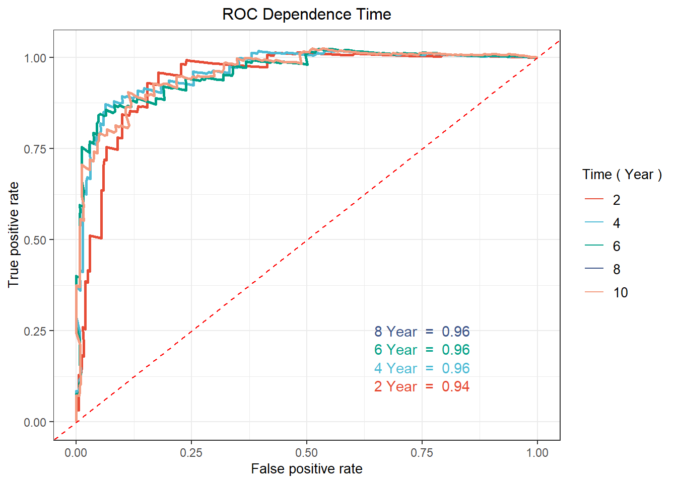
library(grid)时间依赖 ROC
注记
Hiplot 网站
本页面为 Hiplot Time ROC 插件的源码版本教程,您也可以使用 Hiplot 网站实现无代码绘图,更多信息请查看以下链接:
生存分析中受试者操作特征(ROC)与时间记录分析。
环境配置
系统: Cross-platform (Linux/MacOS/Windows)
编程语言: R
依赖包:
plotROC;survivalROC;ggplot2;grid
数据准备
- <表1>:(数字)生存数据(即生存,风险)。
- <表2>:(数字)时间数据。
# 加载数据
data1 <- read.delim("files/Hiplot/171-time-roc-data1.txt", header = T)
data2 <- read.delim("files/Hiplot/171-time-roc-data2.txt", header = T)

# 整理数据格式
surv_table <- data1
colnames(surv_table) <- c("surv", "cens", "risk")
mtime <- as.data.frame(data2)[, 1]
sroc <- lapply(mtime, function(t) {
  stroc <- survivalROC(
    Stime = surv_table$surv,
    status = surv_table$cens,
    marker = surv_table$risk,
    predict.time = t,
    method = "KM"
  )
  data.frame(
    TPF = stroc[["TP"]],
    FPF = stroc[["FP"]],
    cut = stroc[["cut.values"]],
    time = rep(
      stroc[["predict.time"]],
      length(stroc[["TP"]])
    ),
    AUC = rep(
      stroc$AUC,
      length(stroc$FP)
    )
  )
})
mroc <- do.call(rbind, sroc)
mroc$time <- factor(mroc$time)

# 查看数据
head(data1)
surv cens risk
1 11.126027 0 0.19205450
2 9.794521 0 0.47734974
3 13.690411 0 0.04605343
4 10.068493 0 0.29717146
5 3.317808 0 0.18144610
6 12.312329 0 0.62681895head(data2) times
1 2
2 4
3 6
4 8
5 10可视化
# 时间依赖 ROC
col <- c("#E64B35FF","#4DBBD5FF","#00A087FF","#3C5488FF","#F39B7FFF")
p <- ggplot(mroc, aes(x = FPF, y = TPF, label = cut, color = time)) +
  plotROC::geom_roc(labels = FALSE, stat = "identity", n.cuts = 0) +
  geom_abline(slope = 1, intercept = 0, color = "red", linetype = 2) +
  labs(title = "ROC Dependence Time", x = "False positive rate",
       y = "True positive rate",
       color = paste("Time", "(", "Year", ")")) +
  theme_bw() +
  theme(text = element_text(family = "Arial"),
        plot.title = element_text(size = 12, hjust = 0.5),
        axis.title = element_text(size = 10),
        legend.position = "right",
        legend.direction = "vertical",
        legend.title = element_text(size = 10),
        legend.text = element_text(size = 10)) +
  scale_color_manual(values = col)

auc <- levels(factor(mroc$AUC))
for (i in 1:length(auc)) {
  p <- p + annotate("text",
    x = 0.75,
    y = 0.05 + 0.05 * i, ## 注释text的位置
    col = col[i],
    label = paste(
      paste(paste(mtime[i], "Year", sep = " "), " = "),
      round(as.numeric(auc[i]), 2)
    )
  )
}

p