# 安装包
if (!requireNamespace("umap", quietly = TRUE)) {
  install.packages("umap")
}
if (!requireNamespace("ggpubr", quietly = TRUE)) {
  install.packages("ggpubr")
}

# 加载包
library(umap)
library(ggpubr)UMAP
注记
Hiplot 网站
本页面为 Hiplot UMAP 插件的源码版本教程,您也可以使用 Hiplot 网站实现无代码绘图,更多信息请查看以下链接:
UMAP 是一种非线性降维算法,适用于高维数据降维到 2 维或 3 维并进行可视化。该算法能够使较大相似度的点,t 分布在低维空间中的距离更近;而对于低相似度的点,t 分布在低维空间中的距离更远。
环境配置
系统: Cross-platform (Linux/MacOS/Windows)
编程语言: R
依赖包:
umap;ggpubr
数据准备
载入数据为数据集(基因名称及其对应的基因表达值)和样本信息(样本名称及分组)。
# 加载数据
data1 <- read.delim("files/Hiplot/176-umap-data1.txt", header = T)
data2 <- read.delim("files/Hiplot/176-umap-data2.txt", header = T)

# 整理数据格式
sample.info <- data2
rownames(data1) <- data1[, 1]
data1 <- as.matrix(data1[, -1])
## umap
set.seed(123)
umap_info <- umap(t(data1))
colnames(umap_info$layout) <- c("UMAP_1", "UMAP_2")
# handle data
umap_data <- data.frame(
  sample = colnames(data1),
  umap_info$layout
)
colorBy <- sample.info[match(colnames(data1), sample.info[, 1]), "Species"]
colorBy <- factor(colorBy, level = colorBy[!duplicated(colorBy)])
umap_data$colorBy = colorBy
shapeBy <- NULL

# 查看数据
head(data1[,1:5])
M1 M2 M3 M4 M5
Sepal.Length 5.1 4.9 4.7 4.6 5.0
Sepal.Width 3.5 3.0 3.2 3.1 3.6
Petal.Length 1.4 1.4 1.3 1.5 1.4
Petal.Width 0.2 0.2 0.2 0.2 0.2head(data2) Samples Species
1 M1 setosa
2 M2 setosa
3 M3 setosa
4 M4 setosa
5 M5 setosa
6 M6 setosa可视化
# umap
p <- ggscatter(data = umap_data, x = "UMAP_1", y = "UMAP_2", size = 2,
               palette = "lancet", color = "colorBy") +
  labs(color = "group") +
  ggtitle("UMAP Plot") +
  theme_classic() +
  theme(text = element_text(family = "Arial"),
        plot.title = element_text(size = 12,hjust = 0.5),
        axis.title = element_text(size = 12),
        axis.text = element_text(size = 10),
        axis.text.x = element_text(angle = 0, hjust = 0.5,vjust = 1),
        legend.position = "right",
        legend.direction = "vertical",
        legend.title = element_text(size = 10),
        legend.text = element_text(size = 10))

p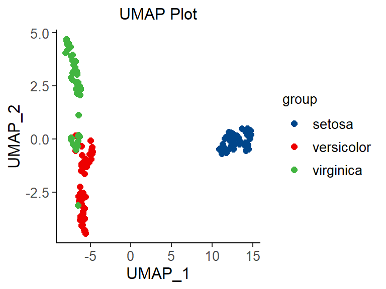
不同颜色表示不同样本,与 PCA(主成分分析)图形解释相同,不同之处在于可视化效果,t-SNE 中对于不相似的点,用一个较小的距离会产生较大的梯度来让这些点排斥开来。