# Install packages
if (!requireNamespace("survival", quietly = TRUE)) {
  install.packages("survival")
}
if (!requireNamespace("rms", quietly = TRUE)) {
  install.packages("rms")
}
if (!requireNamespace("ggplotify", quietly = TRUE)) {
  install.packages("ggplotify")
}

# Load packages
library(survival)
library(rms)
library(ggplotify)Nomogram
Note
Hiplot website
This page is the tutorial for source code version of the Hiplot Nomogram plugin. You can also use the Hiplot website to achieve no code ploting. For more information please see the following link:
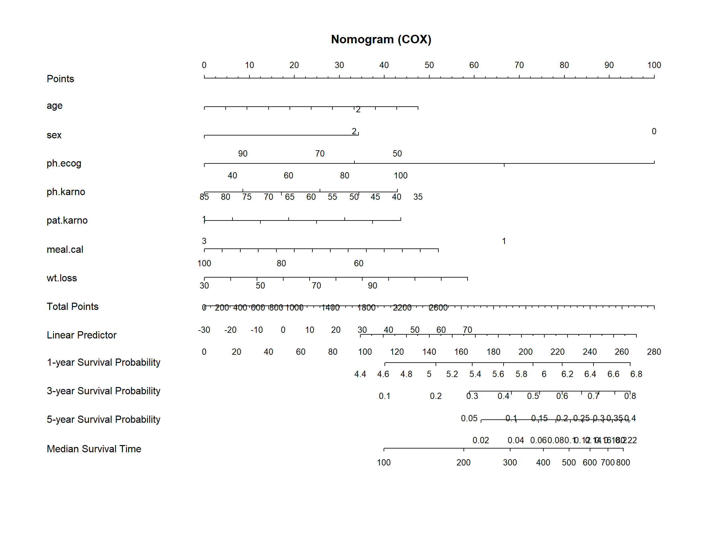
Nomogram is often used to evaluate the prognosis of oncology and medicine, and can visualize the results of logistic regression or Cox regression.
Setup
System Requirements: Cross-platform (Linux/MacOS/Windows)
Programming language: R
Dependent packages:
survival;rms;ggplotify
Data Preparation
Survival data frame with time, which sex and status are presented by number such as 0,1 according to example data.
# Load data
data <- read.delim("files/Hiplot/131-nomogram-data.txt", header = T)

# Convert data structure
dd <- datadist(data)
options(datadist = "dd")
## Build COX model and run nomogram
cox_res <- psm(
  data = data,
  as.formula(paste(
    sprintf("Surv(%s, %s) ~ ", colnames(data)[1], colnames(data)[2]),
    paste(colnames(data)[3:length(colnames(data))],
      collapse = "+"
    )
  )),
  # Surv(time, status) ~ age + sex + ph.ecog + ph.karno + pat.karno,
  dist = "lognormal"
)
## Build survival probability function
surv <- Survival(cox_res)
## Build quantile survival time function
med <- Quantile(cox_res)

cox_nomo <- nomogram(
  cox_res,
  fun = list(function(x) surv(365, x), function(x) surv(1095, x),
             function(x) surv(1825, x), function(x) med(lp = x)),
  funlabel = c("1-year Survival Probability",
               "3-year Survival Probability",
               "5-year Survival Probability",
               "Median Survival Time"),
  maxscale = 100
)

# View data
head(data)
time status age sex ph.ecog ph.karno pat.karno meal.cal wt.loss
1 306 2 74 1 1 90 100 1175 NA
2 455 2 68 1 0 90 90 1225 15
3 1010 1 56 1 0 90 90 NA 15
4 210 2 57 1 1 90 60 1150 11
5 883 2 60 1 0 100 90 NA 0
6 1022 1 74 1 1 50 80 513 0Visualization
# Nomogram
p <- as.ggplot(function() {
  plot(cox_nomo, scale = 1)
  title(main = "Nomogram (COX)")
})

p