PCAtools

Note

Hiplot website

This page is the tutorial for source code version of the Hiplot PCAtools plugin. You can also use the Hiplot website to achieve no code ploting. For more information please see the following link:

https://hiplot.cn/basic/pcatools?lang=en

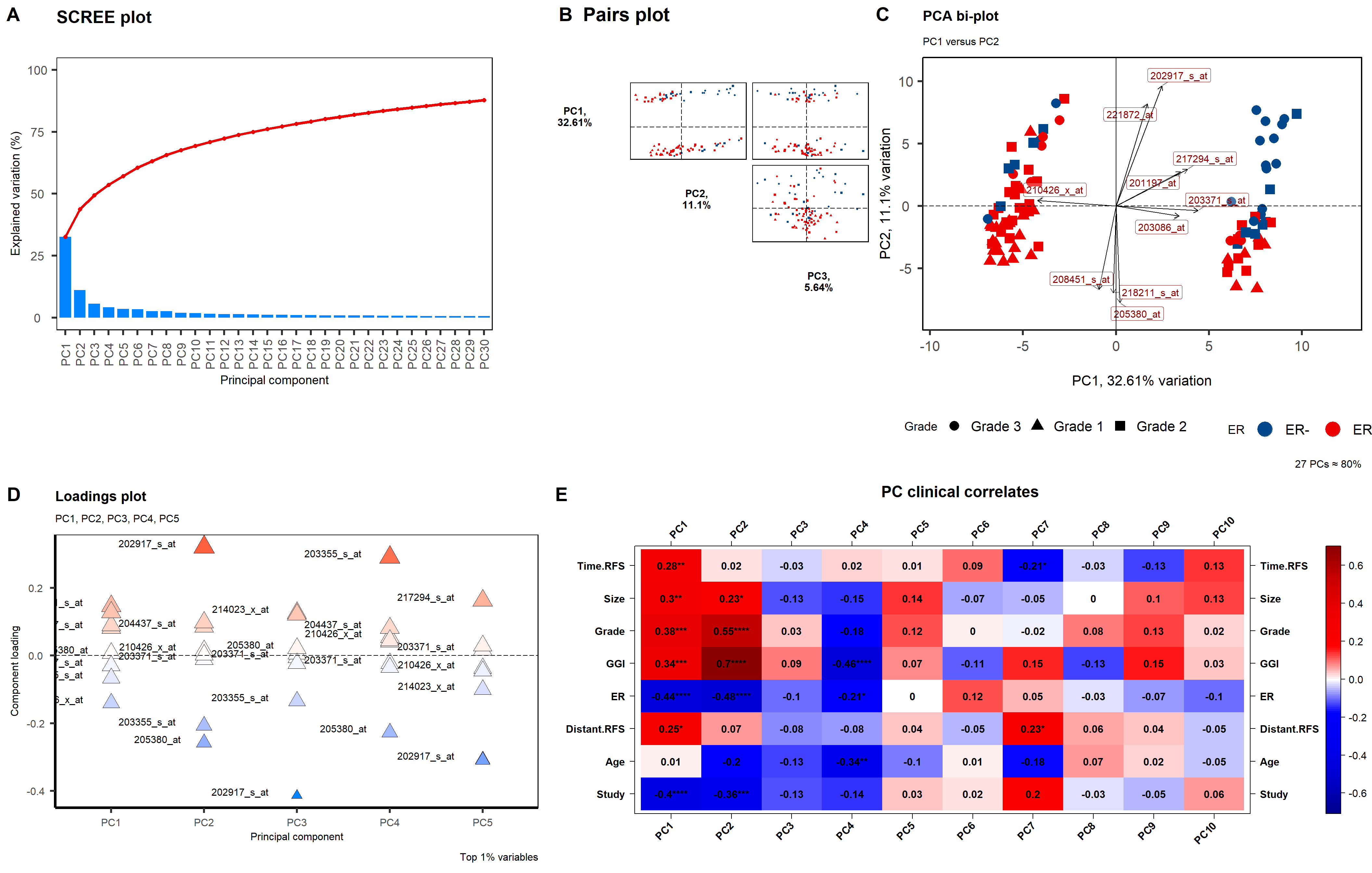
PCAtools can reduce the dimensionality of data through principal component analysis, and view principal component related features at a two-dimensional level

Setup

• System Requirements: Cross-platform (Linux/MacOS/Windows)

• Programming language: R

• Dependent packages: PCAtools; ggplotify; cowplot

# Install packages
if (!requireNamespace("PCAtools", quietly = TRUE)) {
  install_github('kevinblighe/PCAtools')
}
if (!requireNamespace("ggplotify", quietly = TRUE)) {
  install.packages("ggplotify")
}
if (!requireNamespace("cowplot", quietly = TRUE)) {
  install.packages("cowplot")
}

# Load packages
library(PCAtools)
library(ggplotify)
library(cowplot)

Data Preparation

• Data table 1 (numerical matrix):

Each column is a sample, and each row is a feature (such as gene, chip probe).

• Data sheet 2 (sample information):

The first column is the sample, and the other columns are the phenotypic characteristics of the sample, which can be used to mark the color and shape of the point and perform correlation analysis with the principal component.

# Load data
data <- read.delim("files/Hiplot/136-pcatools-data1.txt", header = T)
data2 <- read.delim("files/Hiplot/136-pcatools-data2.txt", header = T)

# View data
head(data[,1:5])

       Probes GSM65752 GSM65753 GSM65755 GSM65757
1   220050_at 6.566843 5.902831 5.185271 5.474453
2 213944_x_at 8.722271 9.088407 9.106401 8.900869
3   215441_at 3.812778 3.852745 3.846690 3.842543
4 214792_x_at 6.499815 6.731196 5.951202 6.578830
5 217251_x_at 6.607354 6.555413 6.715821 6.628053
6   207406_at 3.997302 3.964112 3.836560 3.833057

head(data2)

  Samplename    Study Age Distant.RFS  ER       GGI   Grade Size Time.RFS
1   GSM65752 GSE47561  40           0 ER-  2.480050 Grade 3  1.2     2280
2   GSM65753 GSE47561  46           0 ER+ -0.633592 Grade 1  1.3     2675
3   GSM65755 GSE47561  41           1 ER+  1.043950 Grade 3  3.3      182
4   GSM65757 GSE47561  34           0 ER+  1.059190 Grade 2  1.6     3952
5   GSM65758 GSE47561  46           1 ER+ -1.233060 Grade 2  2.1     1824
6   GSM65760 GSE47561  57           1 ER+  0.679034 Grade 3  2.2      699

Visualization

# PCAtools
## Define the plot function
call_pcatools <- function(datTable, sampleInfo,
                          top_var,
                          screeplotComponents, screeplotColBar,
                          pairsplotComponents,
                          biplotShapeBy, biplotColBy,
                          plotloadingsComponents,
                          plotloadingsLowCol,
                          plotloadingsMidCol,
                          plotloadingsHighCol,
                          eigencorplotMetavars,
                          eigencorplotComponents) {
  row.names(datTable) <- datTable[, 1]
  datTable <- datTable[, -1]
  row.names(sampleInfo) <- sampleInfo[, 1]
  data3 <<- pca(datTable, metadata = sampleInfo, removeVar = (100 - top_var) / 100)

  for (i in c("screeplotComponents", "pairsplotComponents",
              "plotloadingsComponents", "eigencorplotComponents")) {
    if (ncol(data3$rotated) < get(i)) {
      assign(i, ncol(data3$rotated))
    }
  }

  p1 <- PCAtools::screeplot(
    data3,
    components = getComponents(data3, 1:screeplotComponents),
    axisLabSize = 14, titleLabSize = 20,
    colBar = screeplotColBar,
    gridlines.major = FALSE, gridlines.minor = FALSE,
    returnPlot = TRUE
  )

  params_pairsplot <- list(
    data3,
    components = getComponents(data3, c(1:pairsplotComponents)),
    triangle = TRUE, trianglelabSize = 12,
    hline = 0, vline = 0,
    pointSize = 0.8, gridlines.major = FALSE, gridlines.minor = FALSE,
    title = "", plotaxes = FALSE,
    margingaps = unit(c(0.01, 0.01, 0.01, 0.01), "cm"),
    returnPlot = TRUE,
    colkey = c("#00468BFF","#ED0000FF"),
    legendPosition = "none"
  )
  params_biplot <- list(data3,
    showLoadings = TRUE,
    lengthLoadingsArrowsFactor = 1.5,
    sizeLoadingsNames = 4,
    colLoadingsNames = "red4",
    # other parameters
    lab = NULL,
    hline = 0, vline = c(-25, 0, 25),
    vlineType = c("dotdash", "solid", "dashed"),
    gridlines.major = FALSE, gridlines.minor = FALSE,
    pointSize = 5,
    legendLabSize = 16, legendIconSize = 8.0,
    drawConnectors = FALSE,
    title = "PCA bi-plot",
    subtitle = "PC1 versus PC2",
    caption = "27 PCs ≈ 80%",
    returnPlot = TRUE,
    legendPosition = "bottom"
  )
  if (!is.null(biplotShapeBy) && biplotShapeBy != "") {
    params_biplot$shape <- biplotShapeBy
    params_pairsplot$shape <- biplotShapeBy
    t <- params_biplot[[1]]$metadata[,biplotShapeBy]
    params_biplot[[1]]$metadata[,biplotShapeBy] <- factor(t,
      levels = t[!duplicated(t)]
    )
    params_pairsplot[[1]]$metadata[,biplotShapeBy] <- factor(t,
      levels = t[!duplicated(t)]
    )
  }
  if (!is.null(biplotColBy) && biplotColBy != "") {
    params_pairsplot$colby <- biplotColBy
    params_pairsplot$colkey <- c("#00468BFF","#ED0000FF")
    params_biplot$colby <- biplotColBy
    params_biplot$colkey <- c("#00468BFF","#ED0000FF")
    t1 <- params_biplot[[1]]$metadata[,biplotColBy]
    params_biplot[[1]]$metadata[,biplotColBy] <- factor(t1,
      levels = t1[!duplicated(t1)]
    )
    params_pairsplot[[1]]$metadata[,biplotColBy] <- factor(t1,
      levels = t1[!duplicated(t1)]
    )
  }

  p2 <- do.call(PCAtools::pairsplot, params_pairsplot)
  p3 <- do.call(PCAtools::biplot, params_biplot)

  p4 <- PCAtools::plotloadings(
    data3,
    rangeRetain = 0.01, labSize = 4,
    components = getComponents(data3, c(1:plotloadingsComponents)),
    title = "Loadings plot", axisLabSize = 12,
    subtitle = "PC1, PC2, PC3, PC4, PC5",
    caption = "Top 1% variables",
    gridlines.major = FALSE, gridlines.minor = FALSE,
    shape = 24, shapeSizeRange = c(4, 8),
    col = c(plotloadingsLowCol, plotloadingsMidCol, plotloadingsHighCol),
    legendPosition = "none",
    drawConnectors = FALSE,
    returnPlot = TRUE
  )

  if (length(eigencorplotMetavars) > 0 && all(eigencorplotMetavars != "")) {
    metavars <- eigencorplotMetavars
  } else {
    metavars <- colnames(sampleInfo)[2:ncol(sampleInfo)]
  }
  if (length(metavars) == 1 && metavars != colnames(sampleInfo)[1]) {
    metavars <- c(colnames(sampleInfo)[1], metavars)
  } else if (length(metavars) == 1 && metavars == colnames(sampleInfo)[1]) {
    stop('eigencorplotMetavars need >= 2 feature')
  }

  p5 <- PCAtools::eigencorplot(
    data3,
    components = getComponents(data3, 1:eigencorplotComponents),
    metavars = metavars,
    cexCorval = 1.0,
    fontCorval = 2,
    posLab = "all",
    rotLabX = 45,
    scale = TRUE,
    main = "PC clinical correlates",
    cexMain = 1.5,
    plotRsquared = FALSE,
    corFUN = "pearson",
    corUSE = "na.or.complete",
    signifSymbols = c("****", "***", "**", "*", ""),
    signifCutpoints = c(0, 0.0001, 0.001, 0.01, 0.05, 1),
    returnPlot = TRUE
  )

  p6 <- plot_grid(
    p1, p2, p3,
    ncol = 3,
    labels = c("A", "B  Pairs plot", "C"),
    label_fontfamily = "Arial",
    label_fontface = "bold",
    label_size = 22,
    align = "h",
    rel_widths = c(1.10, 0.80, 1.10)
  )

  p7 <- plot_grid(
    p4,
    as.grob(p5),
    ncol = 2,
    labels = c("D", "E"),
    label_fontfamily = "Arial",
    label_fontface = "bold",
    label_size = 22,
    align = "h",
    rel_widths = c(0.8, 1.2)
  )

  p <- plot_grid(
    p6, p7,
    ncol = 1,
    rel_heights = c(1.1, 0.9)
  )

  return(p)
}

## plot
p <- call_pcatools(
  datTable = data,
  sampleInfo = data2,
  biplotColBy = "ER",
  biplotShapeBy = "Grade",
  eigencorplotMetavars = colnames(data2)[-1],
  screeplotComponents = 30,
  pairsplotComponents = 3,
  plotloadingsComponents = 5,
  eigencorplotComponents = 10,
  top_var = 90,
  screeplotColBar = "#0085FF",
  plotloadingsLowCol = "#0085FF",
  plotloadingsMidCol = "#FFFFFF",
  plotloadingsHighCol = "#FF0000"
)

p

Figure 1: PCAtools