Slopegraph

Authors

[Editor] Hu Zheng;

[Contributors]

Note

Hiplot website

This page is the tutorial for source code version of the Hiplot Slopegraph plugin. You can also use the Hiplot website to achieve no code ploting. For more information please see the following link:

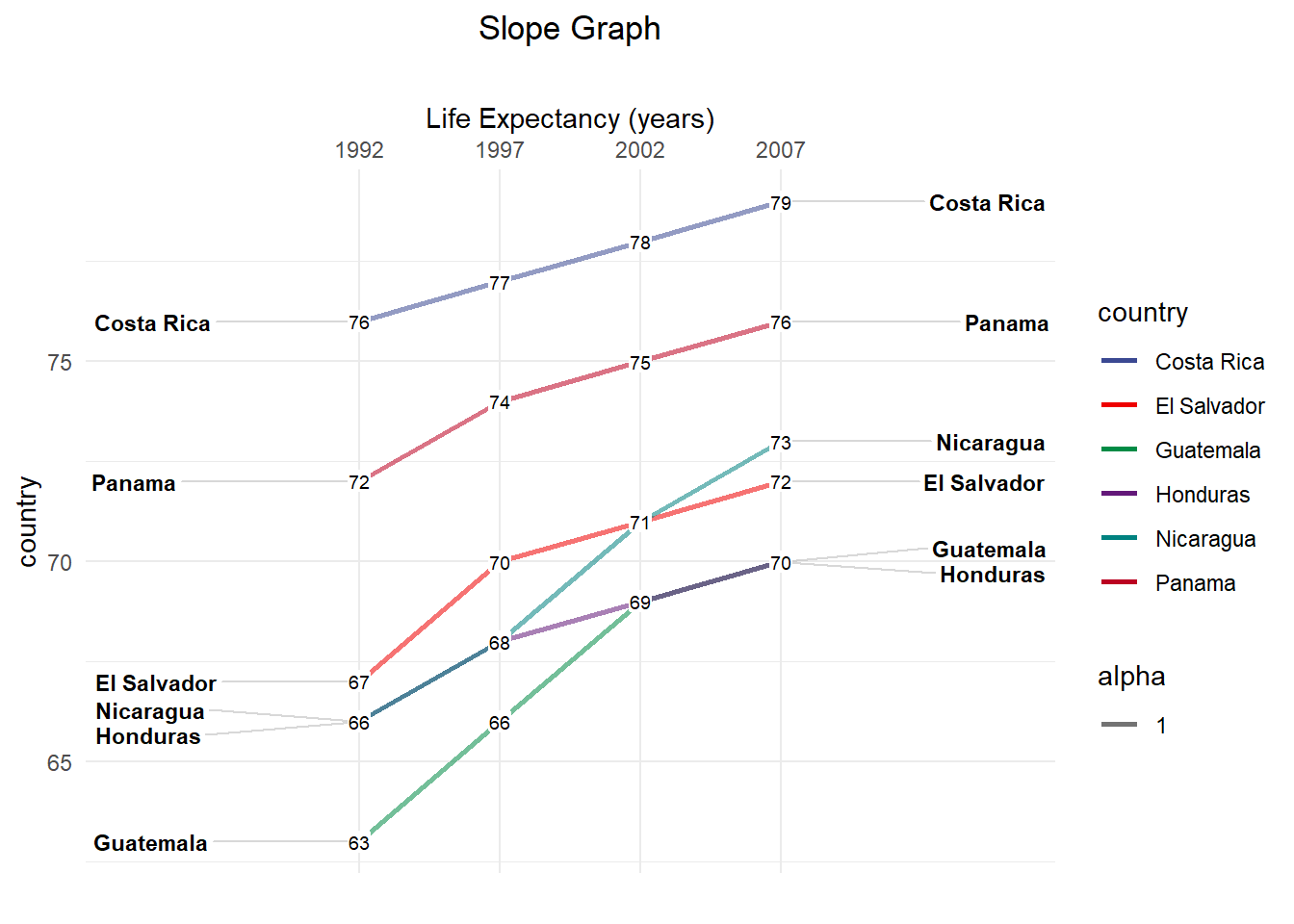
https://hiplot.cn/basic/slopegraph?lang=en

Sopegraph can be used to display the change of values.

Setup

System Requirements: Cross-platform (Linux/MacOS/Windows)
Programming language: R
Dependent packages: CGPfunctions; ggplot2

# Install packages
if (!requireNamespace("CGPfunctions", quietly = TRUE)) {
  install.packages("CGPfunctions")
}
if (!requireNamespace("ggplot2", quietly = TRUE)) {
  install.packages("ggplot2")
}

# Load packages
library(CGPfunctions)
library(ggplot2)

Data Preparation

# Load data
data <- read.delim("files/Hiplot/165-slopegraph-data.txt", header = T)

# convert data structure
data[, "country"] <- factor(data[ ,"country"], levels = unique(data[ ,"country"]))
data[, "year"] <- factor(data[ ,"year"], levels = unique(data[ ,"year"]))

# View data
head(data)

      country continent year lifeExp     pop gdpPercap
1  Costa Rica  Americas 1992      76 3173216  6160.416
2  Costa Rica  Americas 1997      77 3518107  6677.045
3  Costa Rica  Americas 2002      78 3834934  7723.447
4  Costa Rica  Americas 2007      79 4133884  9645.061
5 El Salvador  Americas 1992      67 5274649  4444.232
6 El Salvador  Americas 1997      70 5783439  5154.825

Visualization

# Slopegraph
p <- newggslopegraph(data, year, lifeExp, country) +
  labs(subtitle = "", title = "Slope Graph", x = "Life Expectancy (years)",
       y = "country", caption = "") +
  scale_color_manual(values = c("#3B4992FF", "#EE0000FF", "#008B45FF",
                               "#631879FF", "#008280FF", "#BB0021FF")) +
  theme_minimal() +
  theme(plot.title = element_text(hjust = 0.5))

p