Upset Plot

Note

Hiplot website

This page is the tutorial for source code version of the Hiplot Upset Plot plugin. You can also use the Hiplot website to achieve no code ploting. For more information please see the following link:

https://hiplot.cn/basic/upset-plot?lang=en

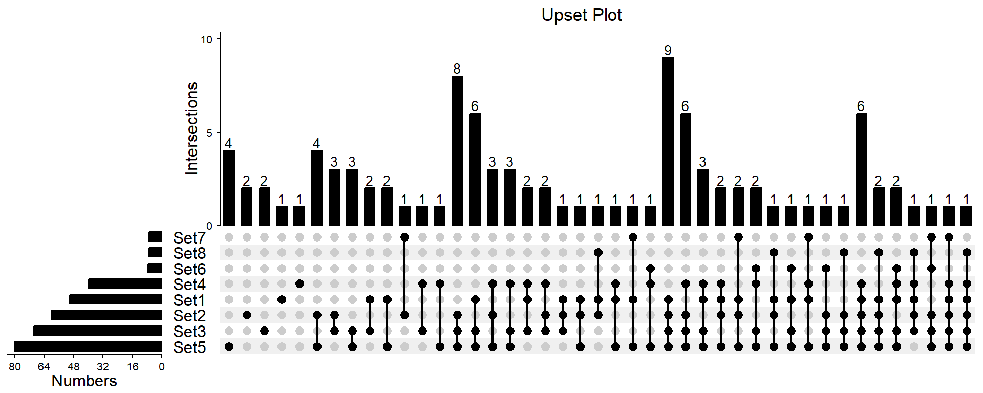
Upset can be used to show the interactive relationship between collections.

Setup

• System Requirements: Cross-platform (Linux/MacOS/Windows)

• Programming language: R

• Dependent packages: VennDiagram; ComplexHeatmap; ggplotify; ggplot2

# Install packages
if (!requireNamespace("VennDiagram", quietly = TRUE)) {
  install.packages("VennDiagram")
}
if (!requireNamespace("ComplexHeatmap", quietly = TRUE)) {
  install_github("jokergoo/ComplexHeatmap")
}
if (!requireNamespace("ggplotify", quietly = TRUE)) {
  install.packages("ggplotify")
}
if (!requireNamespace("ggplot2", quietly = TRUE)) {
  install.packages("ggplot2")
}

# Load packages
library(VennDiagram)
library(ComplexHeatmap)
library(ggplotify)
library(ggplot2)

Data Preparation

There are two types of data tables: list and binary. The list format is that each column is a set and contains all the elements corresponding to the set. In the binary format, the first column is all the elements of all sets, and the subsequent columns are a numeric matrix composed of 0 and 1. 1 indicates that the corresponding row element exists in a certain set, and 0 indicates that it does not exist.

# Load data
data <- read.delim("files/Hiplot/177-upset-plot-data.txt", header = T)

# convert data structure
for (i in seq_len(ncol(data))) {
  data[is.na(data[, i]), i] <- ""
}
data2 <- as.list(data)
data2 <- lapply(data2, function(x) {x[x != ""]})
data2 <- list_to_matrix(data2)
m = make_comb_mat(data2, mode = "distinct")
ss = set_size(m)
cs = comb_size(m)
set_order <- order(ss)
comb_order <- order(comb_degree(m), -cs)

# View data
head(data)

     Set1      Set2     Set3      Set4    Set5      Set6    Set7     Set8
1   ISG15      HES5     DVL1   MATP6P1 FAM132A   FAM132A FAM132A  TNFRSF4
2  TTLL10  AURKAIP1 ARHGEF16   MIR551A    AGRN   MIR551A WBP1LP6   WASH7P
3    HES4 LINC00982   OR4F16  C1orf222 WBP1LP6   MIR200B   PANK4   TMEM52
4  OR4G4P    FAM87B      SKI   MIR200B  KLHL17    ATAD3C  OR4G4P   MMP23B
5 MND2P28       SKI   WASH7P LINC00115  FAM41C   ANKRD65   SSU72   CDK11B
6  FAM87B     GABRD    MEGF6    ATAD3B   PANK4 LINC01128 MND2P28 C1orf170

Visualization

# Upset Plot
p <- as.ggplot(function(){
  top_annotation <- HeatmapAnnotation(
    Intersections = anno_barplot(
      cs, ylim = c(0, max(cs)*1.1), 
      border = FALSE, 
      gp = gpar(fill = "#000000", fontsize = 10), 
      height = unit(5, "cm")
    ), 
    annotation_name_side = "left", 
    annotation_name_rot = 90
  )
  
  left_annotation <- rowAnnotation(
    Numbers = anno_barplot(-ss, axis_param = list(
      at = seq(-max(ss), 0, round(max(ss)/5)),
      labels = rev(seq(0, max(ss), round(max(ss)/5))),
      labels_rot = 0),
      baseline = 0,
      border = FALSE, 
      gp = gpar(fill = "#000000", fontsize = 10), 
      width = unit(4, "cm")
    ),
    set_name = anno_text(set_name(m), location = 0.5,  just = "center",
                         width = max_text_width(set_name(m)) + unit(5, "mm"))
  )
  
  ht = UpSet(m, comb_col = "#000000", bg_col = "#F0F0F0", bg_pt_col = "#CCCCCC",
             pt_size = unit(3, "mm"), lwd = 2, set_order = set_order,
             comb_order = comb_order, top_annotation = top_annotation,
             left_annotation = left_annotation,  right_annotation = NULL,
             show_row_names = FALSE)
  ht = draw(ht)
  od = column_order(ht)
  decorate_annotation("Intersections", {
    grid.text(cs[od], x = seq_along(cs), y = unit(cs[od], "native") + unit(2, "pt"),
              default.units = "native", just = c("left", "bottom"), 
              gp = gpar(fontsize = 10, col = "#000000",
              fontfamily = "Arial"), hjust = 0.5)
  })
})
p <- p + ggtitle("Upset Plot") + 
  theme(plot.title = element_text(hjust = 0.6))

p

Figure 1: Upset Plot