Sankey

Authors

[Editor] Hu Zheng;

[Contributors]

Note

Hiplot website

This page is the tutorial for source code version of the Hiplot Sankey plugin. You can also use the Hiplot website to achieve no code ploting. For more information please see the following link:

https://hiplot.cn/basic/sankey?lang=en

Sankey diagrams are a type of flow diagramin which the width of the arrows is proportional to the flow rate.

Setup

System Requirements: Cross-platform (Linux/MacOS/Windows)
Programming language: R
Dependent packages: ggalluvial; ggplot2

# Install packages
if (!requireNamespace("ggalluvial", quietly = TRUE)) {
  install.packages("ggalluvial")
}
if (!requireNamespace("ggplot2", quietly = TRUE)) {
  install.packages("ggplot2")
}

# Load packages
library(ggalluvial)
library(ggplot2)

Data Preparation

The loaded data are the four variables and the frequency of combination of four variables.

# Load data
data <- read.delim("files/Hiplot/158-sankey-data.txt", header = T)

# Convert data structure
value <- "Freq"
axis <- c("Class", "Sex")
usr_axis <- c()
for (i in seq_len(length(axis))) {
  usr_axis <- c(usr_axis, axis[i])
  assign(paste0("axis", i), axis[i])
}
index_axis <- match(usr_axis, colnames(data))
index_value <- match(value, colnames(data))
data1 <- data[, c(index_value, index_axis)]
## define band color
nlevels <- as.numeric(apply(data1[, -1], 2, function(data) {
  return(length(unique(data)))
}))
band_color <- c("#8DD3C7", "#FFFFB3", "#BEBADA", "#FB8072", "#8DD3C7", "#FFFFB3")
## rename data
data_rename <- data1
colnames(data_rename) <- c(
  "value",
  paste("axis", seq_len(length(usr_axis)), sep = "")
)

# View data
head(data)

  Class    Sex   Age Survived Freq
1   1st   Male Child       No    0
2   2nd   Male Child       No    0
3   3rd   Male Child       No   35
4  Crew   Male Child       No    0
5   1st Female Child       No    0
6   2nd Female Child       No    0

Visualization

# Sankey
p <- ggplot(data_rename, aes(y = value, axis1 = axis1, axis2 = axis2)) +
  geom_alluvium(alpha = 1, aes(fill = data1[, colnames(data1) == "Sex"]),
                width = 0, reverse = FALSE) +
  scale_x_discrete(limits = usr_axis, expand = c(0.02, 0.1)) +
  ylab("") +
  scale_fill_discrete(name = "Sex") +
  coord_flip() +
  geom_stratum(alpha = 1, width = 1 / 8, reverse = FALSE, fill = band_color,
               color = "white") +
  geom_text(stat = "stratum", infer.label = TRUE, reverse = FALSE) +
  ggtitle("Sankey plot") +
  guides(fill = guide_legend(title = "Sex")) +
  scale_fill_manual(values = c("#00468BFF", "#ED0000FF")) +
  theme_bw() +
  theme(text = element_text(family = "Arial"),
        plot.title = element_text(size = 12,hjust = 0.5),
        axis.title = element_text(size = 12),
        axis.text = element_text(size = 10),
        axis.text.x = element_text(angle = 0, hjust = 0.5,vjust = 1),
        legend.position = "right",
        legend.direction = "vertical",
        legend.title = element_text(size = 10),
        legend.text = element_text(size = 10))

p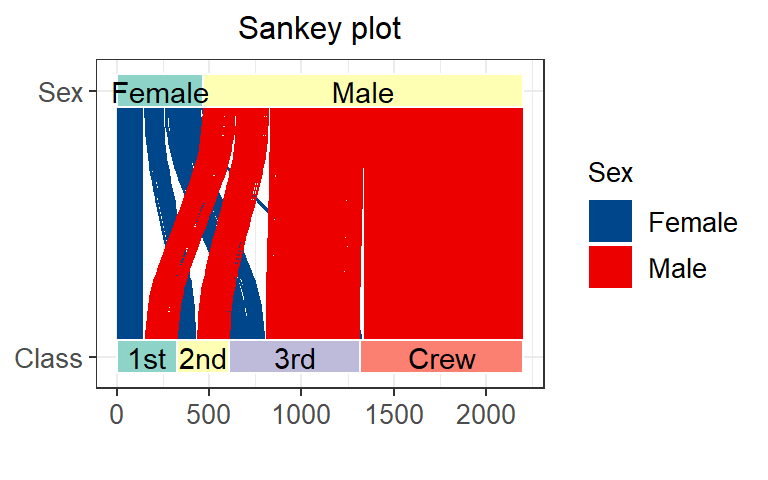

The color of female shunting is blue, the color of male shunting is red, and the width of blue shunting is equal to the total width of female.