Venn

Note

Hiplot website

This page is the tutorial for source code version of the Hiplot Venn plugin. You can also use the Hiplot website to achieve no code ploting. For more information please see the following link:

https://hiplot.cn/basic/venn?lang=en

A Venn diagram is a diagramthat shows all possible logical relations between a finite collection of different sets. These diagrams depict elements as points in the plane, and sets as regions inside closed curves. A Venn diagram consists of multiple overlapping closed curves, usually circles, each representing a set. The points inside a curve labelled S represent elements of the set S, while points outside the boundary represent elements not in the set S. This lends to easily read visualizations; for example, the set of all elements that are members of both sets Sand T, S ∩ T, is represented visually by the area of overlap of the regions S and T. In Venn diagrams the curves are overlapped in every possible way, showing all possible relations between the sets.

Setup

• System Requirements: Cross-platform (Linux/MacOS/Windows)

• Programming language: R

• Dependent packages: VennDiagram; grDevices

# Install packages
if (!requireNamespace("VennDiagram", quietly = TRUE)) {
  install.packages("VennDiagram")
}
if (!requireNamespace("grDevices", quietly = TRUE)) {
  install.packages("grDevices")
}

# Load packages
library(VennDiagram)
library(grDevices)

Data Preparation

The loaded data is a collection of five gene names.

# Load data
data <- read.delim("files/Hiplot/178-venn-data.txt", header = T)

# convert data structure
for (i in seq_len(ncol(data))) {
  data[is.na(data[, i]), i] <- ""
}
raw <- data
data <- as.data.frame(raw[raw[, 1] != "", 1])
colnames(data) <- colnames(raw)[1]
list.num <- 1
for (i in 2:ncol(raw)) {
  if (any(!is.na(raw[, i]) & raw[, i] != "")) {
    tmp <- raw[i]
    tmp <- tmp[tmp[, 1] != "", ]
    tmp <- as.data.frame(tmp)
    colnames(tmp) <- colnames(raw)[i]
    assign(paste0("data", i), tmp)
    list.num <- list.num + 1
  }
}
colnames(data) <- paste("V", seq_len(ncol(data)), sep = "")
colnames(data2) <- paste("V", seq_len(ncol(data2)), sep = "")
colnames(data3) <- paste("V", seq_len(ncol(data3)), sep = "")
colnames(data4) <- paste("V", seq_len(ncol(data4)), sep = "")
colnames(data5) <- paste("V", seq_len(ncol(data5)), sep = "")
data_list <- list(
  n1 = data$V1, n2 = data2$V1, n3 = data3$V1,
  n4 = data4$V1, n5 = data5$V1
)
names(data_list) <- colnames(raw)[1:5]

# View data
head(data)

       V1
1   ISG15
2  TTLL10
3    HES4
4  OR4G4P
5 MND2P28
6  FAM87B

Visualization

# Venn
col <- c("#E64B35FF","#4DBBD5FF","#00A087FF","#3C5488FF","#F39B7FFF")
p <- venn.diagram(
  data_list, scaled = F, euler.d = F, filename = NULL, col = "black",
  fill = col,
  cex = c(
    1.5, 1.5, 1.5, 1.5, 1.5, 1, 0.8, 1, 0.8, 1, 0.8, 1, 0.8,
    1, 0.8, 1, 0.55, 1, 0.55, 1, 0.55, 1, 0.55, 1, 0.55, 1, 1, 1, 1, 1, 1.5
  ),
  cat.col = col, cat.cex = 1,
  main.fontfamily = "Arial", fontfamily = "Arial", cat.fontface = "bold",
  cat.fontfamily = "Arial", margin = 0.1, main = "Vene Plot", alpha = 0.8
);grid::grid.draw(p)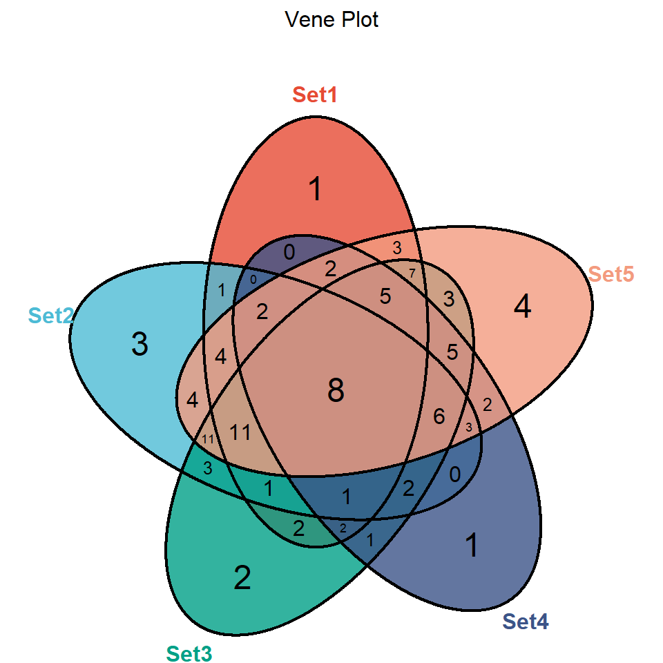

Figure 1: Venn

The closed curve of 5 colors represents 5 sets, and the number represents the number of overlapping or non-overlapping genes in multiple sets. For example, 8 in the sample figure represents 8 identical gene names in 5 sample sets.