# Install packages
if (!requireNamespace("ggplot2", quietly = TRUE)) {
  install.packages("ggplot2")
}
if (!requireNamespace("RColorBrewer", quietly = TRUE)) {
  install.packages("RColorBrewer")
}

# Load packages
library(ggplot2)
library(RColorBrewer)Germany Map
Note
Hiplot website
This page is the tutorial for source code version of the Hiplot Germany Map plugin. You can also use the Hiplot website to achieve no code ploting. For more information please see the following link:
Setup
System Requirements: Cross-platform (Linux/MacOS/Windows)
Programming language: R
Dependent packages:
ggplot2;RColorBrewer
Data Preparation
# Load data
data <- read.delim("files/Hiplot/107-map-germany-data.txt", header = T)
dt_map <- readRDS("files/Hiplot/germany.rds")
# Convert data structure
dt_map$Value <- data$value[match(dt_map$ENG_NAME, data$name)]
# View data
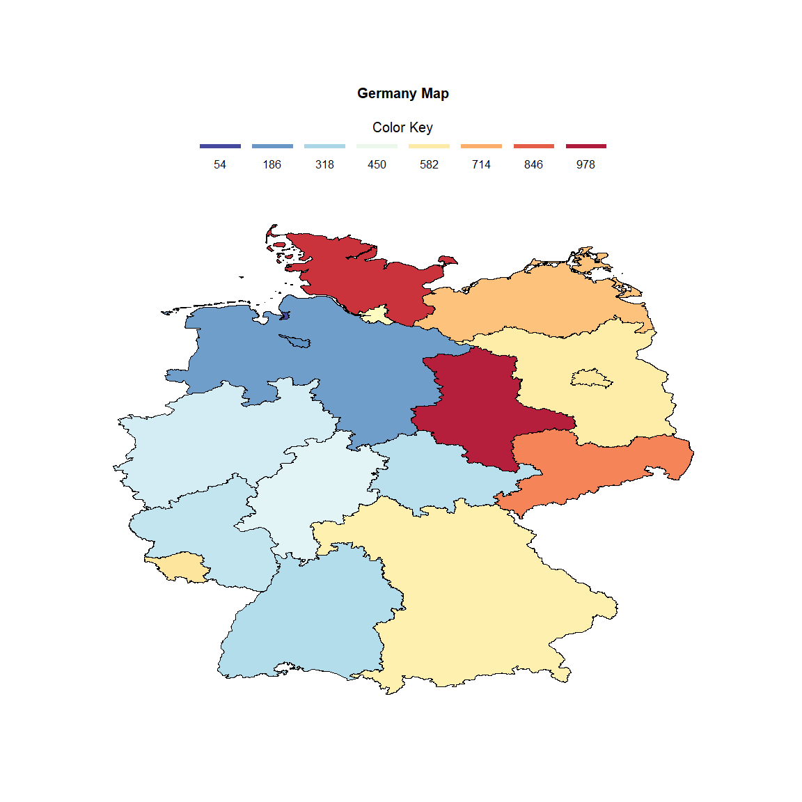
head(data) name value
1 Baden-Württemberg 334
2 Bayern 562
3 Berlin 980
4 Brandenburg 577
5 Bremen 54
6 Hamburg 528Visualization
# Germany Map
p <- ggplot(dt_map) +
  geom_polygon(aes(x = long, y = lat, group = group, fill = Value),
               alpha = 0.9, size = 0.5) +
  geom_path(aes(x = long, y = lat, group = group), color = "black", size = 0.2) +
  scale_fill_gradientn(
    colours = colorRampPalette(rev(brewer.pal(11,"RdYlBu")))(500),
    breaks = seq(min(data$value), max(data$value),
                 round((max(data$value)-min(data$value))/7)),
    name = "Color Key",
    guide = guide_legend(
      direction = "vertical", keyheight = unit(1, units = "mm"),
      keywidth = unit(8, units = "mm"),
      title.position = "top", title.hjust = 0.5, label.hjust = 0.5,
      nrow = 1, byrow = T, reverse = F, label.position = "bottom")) +
  theme(text = element_text(color = "#3A3F4A"),
        axis.text = element_blank(),
        axis.ticks = element_blank(),
        panel.grid.major = element_blank(),
        panel.grid.minor = element_blank(),
        legend.position = "top",
        legend.text = element_text(size = 4 * 1.5, color = "black"),
        legend.title = element_text(size = 5 * 1.5, color = "black"),
        plot.title = element_text(
          face = "bold", size = 5 * 1.5, hjust = 0.5,
          margin = margin(t = 4, b = 5), color = "black"),
        plot.background = element_rect(fill = "#FFFFFF", color = "#FFFFFF"),
        panel.background = element_rect(fill = "#FFFFFF", color = NA),
        legend.background = element_rect(fill = "#FFFFFF", color = NA),
        plot.margin = unit(c(1.5, 1.5, 1.5, 1.5), "cm")) +
  labs(x = NULL, y = NULL, title = "Germany Map")

p