Stack Violin

Note

Hiplot website

This page is the tutorial for source code version of the Hiplot Stack Violin plugin. You can also use the Hiplot website to achieve no code ploting. For more information please see the following link:

https://hiplot.cn/basic/stack-violin?lang=en

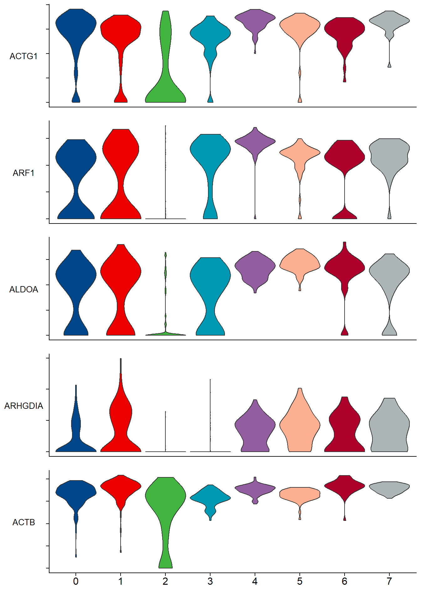
The expression of key genes in each cluster in single-cell transcriptomic (Single Cell RNA-Seq)analysis.

Setup

• System Requirements: Cross-platform (Linux/MacOS/Windows)

• Programming language: R

• Dependent packages: limma; Seurat; ggplot2

# Install packages
if (!requireNamespace("limma", quietly = TRUE)) {
  install.packages("limma")
}
if (!requireNamespace("Seurat", quietly = TRUE)) {
  install.packages("Seurat")
}
if (!requireNamespace("ggplot2", quietly = TRUE)) {
  install.packages("ggplot2")
}

# Load packages
library(limma)
library(Seurat)
library(ggplot2)

Data Preparation

Gene expression matrix. Gene expression matrix in all cells and groups in single cell transcriptome analysis (Single Cell RNA-Seq).

# Load data
data <- read.delim("files/Hiplot/166-stack-violin-data.txt", header = T)

# convert data structure
data <- as.matrix(data)
rownames(data) <- data[, 1]
exp <- data[, 2:ncol(data)]
dimnames <- list(
  rownames(exp),
  colnames(exp)
)
data <- matrix(as.numeric(as.matrix(exp)),
  nrow = nrow(exp),
  dimnames = dimnames
)
data <- avereps(data,
  ID = rownames(data)
)
## Convert the matrix to a Seurat object and filter the data
pbmc <- CreateSeuratObject(
  counts = data,
  project = "seurat",
  min.cells = 0,
  min.features = 0,
  names.delim = "_",
)
## Calculate the percentage of mitochondrial genes using the PercentageFeatureSet function
pbmc[["percent.mt"]] <- PercentageFeatureSet(
  object = pbmc,
  pattern = "^MT-"
)
## Filter the data
pbmc <- subset(
  x = pbmc,
  subset = nFeature_RNA > 50 & percent.mt < 5
)
## Normalize the data
pbmc <- NormalizeData(
  object = pbmc,
  normalization.method = "LogNormalize",
  scale.factor = 10000, verbose = F
)
## Extract genes with large coefficient of variation between cells
pbmc <- FindVariableFeatures(
  object = pbmc,
  selection.method = "vst",
  nfeatures = 1500, verbose = F
)
## Standard preprocessing steps before PCA dimensionality reduction
pbmc <- ScaleData(pbmc)
pbmc <- RunPCA(
  object = pbmc,
  npcs = 20,
  pc.genes = VariableFeatures(object = pbmc)
)
## Distribution of p-values for each PC and uniform distribution
pbmc <- JackStraw(
  object = pbmc,
  num.replicate = 100
)
pbmc <- ScoreJackStraw(
  object = pbmc,
  dims = 1:20
)
## Calculate neighbor distance
pbmc <- FindNeighbors(
  object = pbmc,
  dims = 1:20
)
## Group cells and optimize standard modularity
pbmc <- FindClusters(
  object = pbmc,
  resolution = 0.5
)

Modularity Optimizer version 1.3.0 by Ludo Waltman and Nees Jan van Eck

Number of nodes: 653
Number of edges: 18908

Running Louvain algorithm...
Maximum modularity in 10 random starts: 0.8684
Number of communities: 8
Elapsed time: 0 seconds

## TSNE clustering
pbmc <- RunTSNE(
  object = pbmc,
  dims = 1:20
)
## Finding differentially expressed features
log_fc_filter <- 0.5
adj_pval_filter <- 0.05
pbmc_markers <- FindAllMarkers(
  object = pbmc,
  only.pos = FALSE,
  min.pct = 0.25,
  logfc.threshold = log_fc_filter
)
pbmc_sig_markers <- pbmc_markers[(abs(as.numeric(
  as.vector(pbmc_markers$avg_logFC)
)) > log_fc_filter &
  as.numeric(as.vector(pbmc_markers$p_val_adj)) <
    adj_pval_filter), ]

# View data
head(data[,1:5])

         PT089_P1_A01 PT089_P1_A02 PT089_P1_A03 PT089_P1_A04 PT089_P1_A05
A1BG             0.00            0            0            0            0
A1BG-AS1         0.00            0            0            0            0
A1CF             0.00            0            0            1            0
A2M              0.00            0            0          339            0
A2M-AS1          0.00            0            0            0            0
A2ML1            1.08            0            0            0            0

Visualization

# Stack Violin
## Define the plot function
modify_vlnplot <- function(obj,
                           feature,
                           pt.size = 0,
                           plot.margin = unit(c(-0.75, 0, -0.75, 0), "cm"),
                           ...) {
  p <- VlnPlot(obj,
    features = feature,
    pt.size = pt.size,
    ...
  )

  p <- p +
    xlab("") +
    ylab(feature) +
    theme(
      axis.text.x = element_blank(),
      axis.text.y = element_blank(),
      axis.ticks.x = element_blank(),
      axis.ticks.y = element_line(),
      axis.title.y = element_text(angle = 0, vjust = 0.5),
      plot.margin = plot.margin,
      text = element_text(
        family = "Arial"
      ),
      plot.title = element_blank(),
      axis.title = element_text(
        size = 10
      ),
      legend.position = "none",
      legend.direction = "vertical",
      legend.title = element_text(
        size = 10
      ),
      legend.text = element_text(
        size = 10
      )
    ) +
    scale_fill_manual(values = c("#00468BFF","#ED0000FF","#42B540FF","#0099B4FF",
                                 "#925E9FFF","#FDAF91FF","#AD002AFF","#ADB6B6FF"))
  return(p)
}

## main function
stacked_vln_plot <- function(obj,
                           features,
                           pt.size = 0,
                           plot.margin = unit(c(-0.75, 0, -0.75, 0), "cm"),
                           ...) {
  plot_list <- purrr::map(
    features,
    function(x) {
      modify_vlnplot(
        obj = obj,
        feature = x,
        ...
      )
    }
  )
  plot_list[[length(plot_list)]] <- plot_list[[length(plot_list)]] +
    theme(
      axis.text.x = element_text(),
      axis.ticks.x = element_line()
    )
  p <- patchwork::wrap_plots(
    plotlist = plot_list,
    ncol = 1
  )
  return(p)
}

## plot
p <- stacked_vln_plot(pbmc, c("ACTG1","ARF1","ALDOA","ARHGDIA","ACTB"), pt.size = 0)

p

Figure 1: Stack Violin