# Install packages
if (!requireNamespace("scatterpie", quietly = TRUE)) {
  install.packages("scatterpie")
}

# Load packages
library(scatterpie)Scatterpie
Note
Hiplot website
This page is the tutorial for source code version of the Hiplot Scatterpie plugin. You can also use the Hiplot website to achieve no code ploting. For more information please see the following link:
Scatter Pie can be used to visualize data fraction in different space coordinates.
Setup
System Requirements: Cross-platform (Linux/MacOS/Windows)
Programming language: R
Dependent packages:
scatterpie
Data Preparation
# Load data
data <- read.delim("files/Hiplot/163-scatterpie-data.txt", header = T)

# View data
head(data)
x y A B C D
1 -56.047565 12.665926 0.71040656 2.887786 1.309570 2.892264
2 -23.017749 -1.427338 0.25688371 1.403569 1.375096 4.945092
3 7.050839 68.430114 0.24669188 0.524395 3.189978 5.138863
4 12.928774 -11.288549 0.34754260 3.144288 3.789556 2.295894
5 -126.506123 29.230687 0.95161857 3.029335 1.048951 2.471943
6 -68.685285 6.192712 0.04502772 3.203072 2.596539 4.439393Visualization
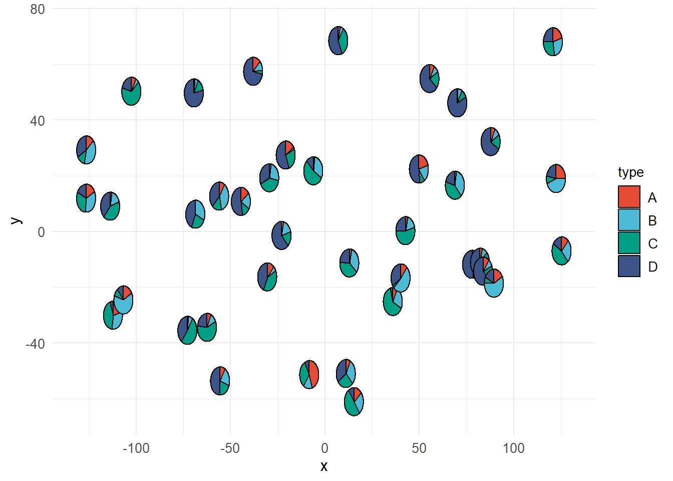
# Scatterpie
p <- ggplot() +
  geom_scatterpie(data = data, aes(x = x, y = y), cols = colnames(data)[-c(1, 2)]) +
  scale_fill_manual(values = c("#E64B35FF","#4DBBD5FF","#00A087FF","#3C5488FF")) +
  labs(x="x", y="y") +
  theme_minimal() +
  theme(text = element_text(family = "Arial"),
        plot.title = element_text(size = 12,hjust = 0.5),
        axis.title = element_text(size = 12),
        axis.text = element_text(size = 10),
        axis.text.x = element_text(angle = 0, hjust = 0.5,vjust = 1),
        legend.position = "right",
        legend.direction = "vertical",
        legend.title = element_text(size = 10),
        legend.text = element_text(size = 10))

p