Volcano

Authors

[Editor] Hu Zheng;

[Contributors]

Note

Hiplot website

This page is the tutorial for source code version of the Hiplot Volcano plugin. You can also use the Hiplot website to achieve no code ploting. For more information please see the following link:

https://hiplot.cn/basic/volcano?lang=en

The volcanogram is a visual representation of the difference in gene expression between two samples.

Setup

System Requirements: Cross-platform (Linux/MacOS/Windows)
Programming language: R
Dependent packages: ggpubr

# Install packages
if (!requireNamespace("ggpubr", quietly = TRUE)) {
  install.packages("ggpubr")
}

# Load packages
library(ggpubr)

Data Preparation

The loaded data is the gene name and its corresponding logFC and p.value.

# Load data
data <- read.delim("files/Hiplot/183-volcano-data.txt", header = T)

# convert data structure
## Perform log10 transformation on the difference p (adj.P.Val column)
data[, "logP"] <- -log10(as.numeric(data[, "P.Value"]))
data[, "logFC"] <- as.numeric(data[, "logFC"])
## Add a new column Group
data[, "Group"] <- "not-significant"
## Up and down
data$Group[which((data[, "P.Value"] < 0.05) & (data$logFC >= 2))] <- "Up-regulated"
data$Group[which((data[, "P.Value"] < 0.05) & (data$logFC <= 2 * -1))] <- "Down-regulated"
## Add a new column Label
data[["Label"]] <- ""
## Sort the p-values of differentially expressed genes from small to large
data <- data[order(data[, "P.Value"]), ]
## Among the highly expressed genes, select the 10 with the smallest adj.P.Val
up_genes <- head(data[, "Symbol"][which(data$Group == "Up-regulated")], 10)
down_genes <- head(data[, "Symbol"][which(data$Group == "Down-regulated")], 10)
not_sig_genes <- NA
## Merge up_genes and down_genes and add them to Label
deg_top_genes <- c(as.character(up_genes), as.character(not_sig_genes),
as.character(down_genes))
deg_top_genes <- deg_top_genes[!is.na(deg_top_genes)]
data$Label[match(deg_top_genes, data[, "Symbol"])] <- deg_top_genes

# View data
head(data)

    Symbol     logFC  P.Value     logP           Group    Label
1      LTB  2.580831 1.17e-14 13.93181    Up-regulated      LTB
2    CDCA5 -2.326302 2.46e-13 12.60906  Down-regulated    CDCA5
3 C10orf54  3.307901 3.53e-13 12.45223    Up-regulated C10orf54
4    CAPN7  2.514235 1.04e-12 11.98297    Up-regulated    CAPN7
5     OIP5 -2.166620 1.43e-12 11.84466  Down-regulated     OIP5
7     PKIG -1.560504 1.58e-12 11.80134 not-significant

Visualization

# Volcano
options(ggrepel.max.overlaps = 100)
p <- ggscatter(data, x = "logFC", y = "logP", color = "Group", 
               palette = c("#2f5688", "#BBBBBB", "#CC0000"), size = 1, 
               alpha = 0.5, font.label = 8, repel = TRUE, label=data$Label,
               xlab = "log2(Fold Change)", ylab = "-log10(P Value)",
               show.legend.text = FALSE) +
  ggtitle("Volcano Plot") +
  geom_hline(yintercept = -log(0.05, 10), linetype = "dashed") +
  geom_vline(xintercept = c(2, -2), linetype = "dashed") +
  theme_bw() +
  theme(text = element_text(family = "Arial"),
        plot.title = element_text(size = 12,hjust = 0.5),
        axis.title = element_text(size = 12),
        axis.text = element_text(size = 10),
        axis.text.x = element_text(angle = 0, hjust = 0.5,vjust = 1),
        legend.position = "right",
        legend.direction = "vertical",
        legend.title = element_text(size = 10),
        legend.text = element_text(size = 10))

p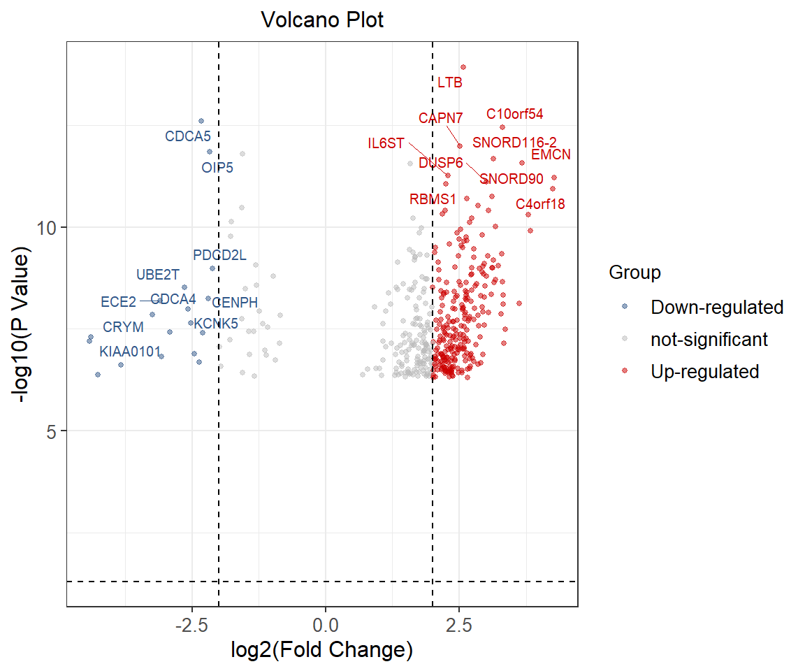

The horizontal axis is denoted by log2 (fold change), and the more different genes are distributed at both ends of the picture.The ordinate is denoted by -log10 (p.value) and is the negative log of the P value of T test significance.Blue dots represent down-regulated genes, red dots represent up-regulated genes, and gray dots represent genes that are not significantly different.