# Install packages
if (!requireNamespace("rms", quietly = TRUE)) {
  install.packages("rms")
}
if (!requireNamespace("survival", quietly = TRUE)) {
  install.packages("survival")
}
if (!requireNamespace("ggplot2", quietly = TRUE)) {
  install.packages("ggplot2")
}
if (!requireNamespace("stringr", quietly = TRUE)) {
  install.packages("stringr")
}

# Load packages
library(rms)
library(survival)
library(ggplot2)
library(stringr)RCS-COX
Note
Hiplot website
This page is the tutorial for source code version of the Hiplot RCS-COX plugin. You can also use the Hiplot website to achieve no code ploting. For more information please see the following link:
Nonlinear regression analysis.
Setup
System Requirements: Cross-platform (Linux/MacOS/Windows)
Programming language: R
Dependent packages:
rms;survival;ggplot2;stringr
Data Preparation
# Load data
data <- read.delim("files/Hiplot/151-rcs-cox-data.txt", header = T)

# Convert data structure
data <- na.omit(data)
ex <- set::not(colnames(data), c("main", "time", "event"))
ex <- str_c(ex, collapse = "+")
dd <<- datadist(data)
options(datadist = "dd")
for (i in 3:5) {
  fit <- coxph(as.formula(paste0("Surv(time, event) ~ rcs(main, nk = i, inclx = T)+", ex, collapse = "+")), data = data, x = TRUE)
  tmp <- extractAIC(fit)
  if (i == 3) {
    AIC <- tmp[2]
    nk <<- 3
  }
  if (tmp[2] < AIC) {
    AIC <- tmp[2]
    nk <<- i
  }
}
fit <- cph(as.formula(paste0("Surv(time, event) ~ rcs(main, nk = nk, inclx = T)+", ex, collapse = "+")), data = data, x = TRUE)
dd$limits$main[2] <- median(data$main)
fit <- update(fit)
orr <- Predict(fit, main, fun = exp, ref.zero = TRUE)

# View data
head(data)
main x1 x2 time event
1 25.54051 1 1 2178 0
2 24.02398 1 2 2172 0
3 22.14290 1 3 2190 0
4 26.63187 1 4 297 1
5 24.41255 1 5 2131 0
6 23.24236 1 6 1 1Visualization
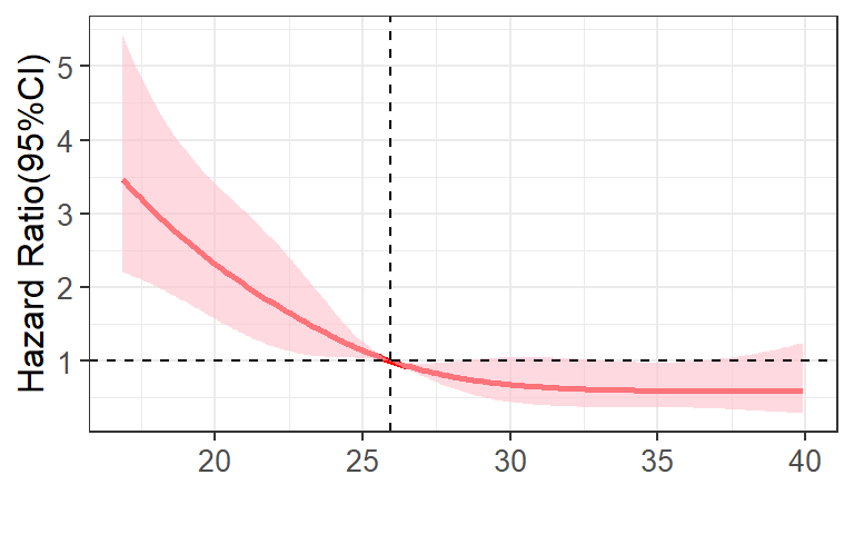
# RCS-COX
p <- ggplot() +
  geom_line(data = orr, aes(main, yhat), linetype = "solid", size = 1, alpha = 1,
            colour = "#FF0000") +
  geom_ribbon(data = orr, aes(main, ymin = lower, ymax = upper), alpha = 0.6,
              fill = "#FFC0CB") +
  geom_hline(yintercept = 1, linetype = 2, size = 0.5) +
  geom_vline(xintercept = dd$limits$main[2], linetype = 2, size = 0.5) +
  labs(x = " ", y = "Hazard Ratio(95%CI)") +
  theme_bw() +
  theme(text = element_text(family = "Arial"),
        plot.title = element_text(size = 12,hjust = 0.5),
        axis.title = element_text(size = 12),
        axis.text = element_text(size = 10),
        axis.text.x = element_text(angle = 0, hjust = 0.5,vjust = 1),
        legend.position = "right",
        legend.direction = "vertical",
        legend.title = element_text(size = 10),
        legend.text = element_text(size = 10))

p