# Install packages
if (!requireNamespace("openair", quietly = TRUE)) {
  install.packages("openair")
}

# Load packages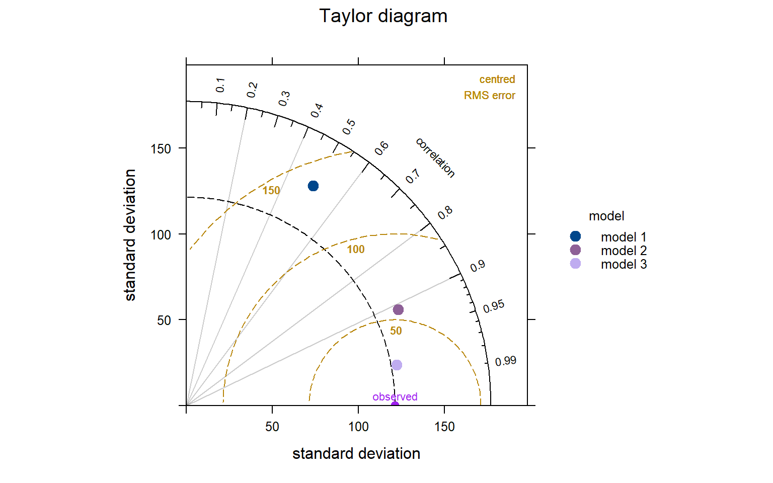
library(openair)Taylor Diagram
Note
Hiplot website
This page is the tutorial for source code version of the Hiplot Taylor Diagram plugin. You can also use the Hiplot website to achieve no code ploting. For more information please see the following link:
It can be used to display the standard deviation (SD), root mean square (RMS) error and correlation coefficient of the models simultaneously.
Setup
System Requirements: Cross-platform (Linux/MacOS/Windows)
Programming language: R
Dependent packages:
openair
Data Preparation
# Load data
dat <- selectByDate(mydata, year = 2003)

# convert data structure
dat <- data.frame(date = mydata$date, obs = mydata$nox, mod = mydata$nox)
dat <- transform(dat, month = as.numeric(format(date, "%m")))
mod1 <- transform(dat, mod = mod + 10 * month + 10 * month * rnorm(nrow(dat)),
model = "model 1")
mod1 <- transform(mod1, mod = c(mod[5:length(mod)], mod[(length(mod) - 3) :
length(mod)]))
mod2 <- transform(dat, mod = mod + 7 * month + 7 * month * rnorm(nrow(dat)),
model = "model 2")
mod3 <- transform(dat, mod = mod + 3 * month + 3 * month * rnorm(nrow(dat)),
model = "model 3")
mod.dat <- rbind(mod1, mod2, mod3)

# View data
head(mod.dat)
date obs mod month model
1 1998-01-01 00:00:00 285 479.8569 1 model 1
2 1998-01-01 01:00:00 NA 255.9534 1 model 1
3 1998-01-01 02:00:00 NA 187.8233 1 model 1
4 1998-01-01 03:00:00 493 207.7949 1 model 1
5 1998-01-01 04:00:00 468 162.2531 1 model 1
6 1998-01-01 05:00:00 264 124.6797 1 model 1Visualization
# Taylor Diagram
TaylorDiagram(mod.dat, obs = "obs", mod = "mod", group = "model",
              main = "Taylor diagram",
              cols = c("#00468BFF","#8e6097","#BFACF0FF"))