Mosaic Ratio Plot

Authors

[Editor] Hu Zheng;

[Contributors]

Note

Hiplot website

This page is the tutorial for source code version of the Hiplot Mosaic Ratio Plot plugin. You can also use the Hiplot website to achieve no code ploting. For more information please see the following link:

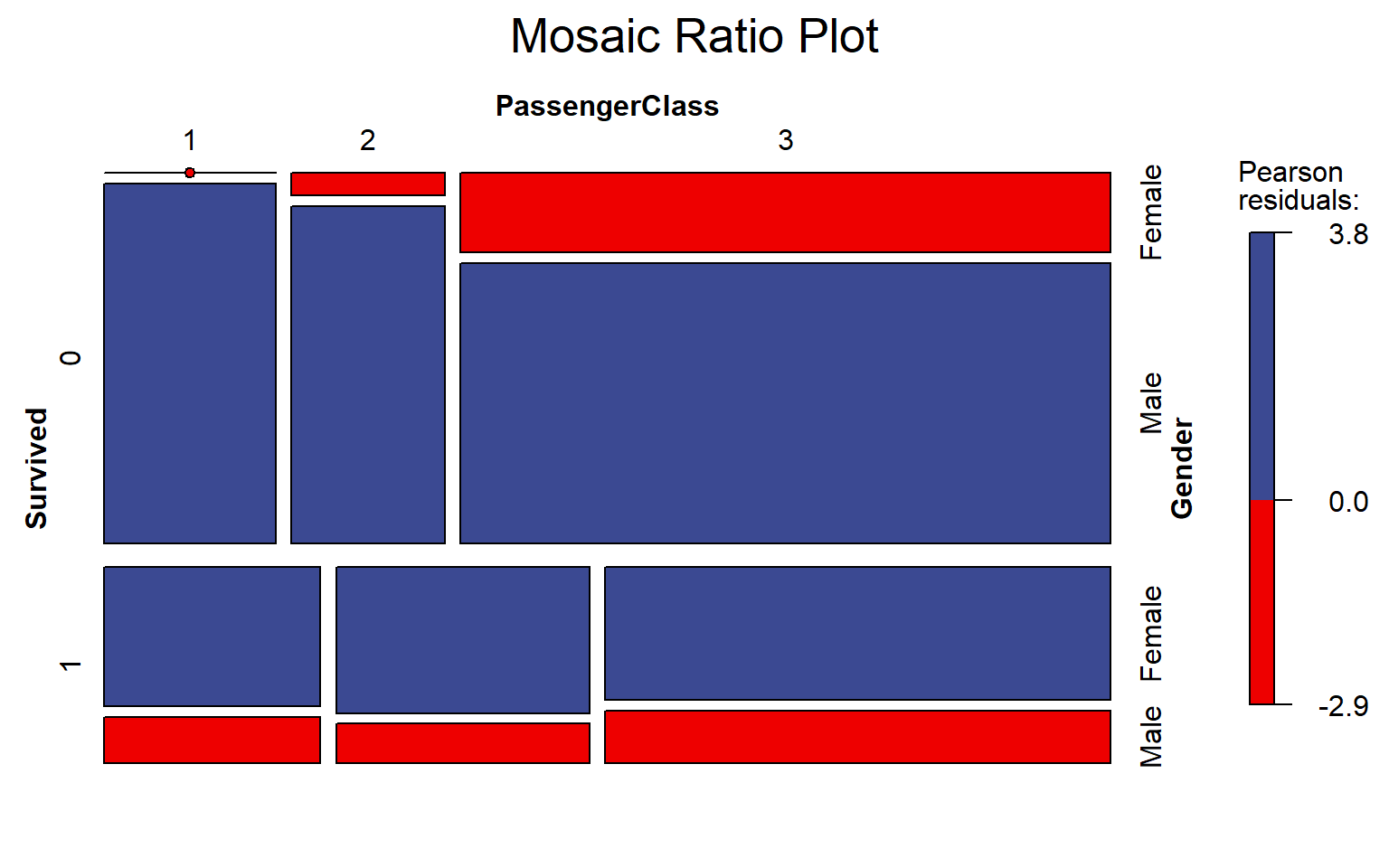
https://hiplot.cn/basic/mosaic?lang=en

Use mosaic blocks to show data proportions.

Setup

System Requirements: Cross-platform (Linux/MacOS/Windows)
Programming language: R
Dependent packages: vcd; DescTools; ggplotify

# Install packages
if (!requireNamespace("vcd", quietly = TRUE)) {
  install.packages("vcd")
}
if (!requireNamespace("DescTools", quietly = TRUE)) {
  install.packages("DescTools")
}
if (!requireNamespace("ggplotify", quietly = TRUE)) {
  install.packages("ggplotify")
}

# Load packages
library(vcd)
library(DescTools)
library(ggplotify)

Data Preparation

# Load data
data <- read.delim("files/Hiplot/123-mosaic-data.txt", header = T)

# Convert data structure
tbl <- xtabs(~ Survived + PassengerClass + Gender, data)

# View data
head(data)

  PassengerId Survived PassengerClass
1           1        0              3
2           2        1              1
3           3        1              3
4           4        1              1
5           5        0              3
6           6        0              3
                                                 Name Gender Age SibSp Parch
1                             Braund, Mr. Owen Harris   Male  22     1     0
2 Cumings, Mrs. John Bradley (Florence Briggs Thayer) Female  38     1     0
3                              Heikkinen, Miss. Laina Female  26     0     0
4        Futrelle, Mrs. Jacques Heath (Lily May Peel) Female  35     1     0
5                            Allen, Mr. William Henry   Male  35     0     0
6                                    Moran, Mr. James   Male  NA     0     0
            Ticket    Fare Cabin Embarked
1        A/5 21171  7.2500  <NA>        S
2         PC 17599 71.2833   C85        C
3 STON/O2. 3101282  7.9250  <NA>        S
4           113803 53.1000  C123        S
5           373450  8.0500  <NA>        S
6           330877  8.4583  <NA>        Q

Visualization

# Mosaic Ratio Plot
p <- as.ggplot(function() {
  mosaic(tbl, shade = TRUE, legend = TRUE, main = "Mosaic Ratio Plot",
         gp = shading_binary(tbl, col = c("#3B4992FF","#EE0000FF")))
})

p